Labs portal
From CSDMS
Labs
CSDMS Workbench: Basic Model Interface (BMI)
Stand alone module
The Basic Model Interface (BMI) is a set of standard control and query functions that, when added to a model code, make that model both easier to learn and easier to couple with other software elements. This lab illustrates how to run a model through its BMI.
Stand alone module
The Basic Model Interface (BMI) is a set of standard control and query functions that, when added to a model code, make that model both easier to learn and easier to couple with other software elements. This lab illustrates how to run a model through its BMI.
Duration:
1.0 hrs
Model used:
Heat
1.0 hrs
Model used:
Heat
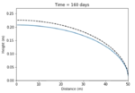
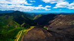
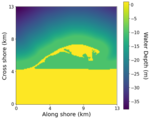
Exploring a shallow unconfined aquifer
Stand alone module
The notebook-based lab uses a simple numerical model to explore how hydraulic conductivity and recharge influence the depth of an unconfined aquifer and the shape of its water table.
Stand alone module
The notebook-based lab uses a simple numerical model to explore how hydraulic conductivity and recharge influence the depth of an unconfined aquifer and the shape of its water table.
Duration:
1.0 hrs
Model used:
(self-contained)
1.0 hrs
Model used:
(self-contained)
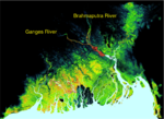
Future Sediment Flux of the Ganges River
Stand alone module
Investigate river sediment supply of the monsoon-driven Ganges River. Explore the effects of future climate changes. Validate a model against observations and discuss uncertainty.
Stand alone module
Investigate river sediment supply of the monsoon-driven Ganges River. Explore the effects of future climate changes. Validate a model against observations and discuss uncertainty.
Duration:
1.0 hrs
Model used:
HydroTrend
1.0 hrs
Model used:
HydroTrend
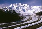
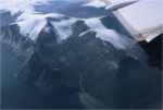
Exploring the growth and retreat of a valley glacier
Stand alone module
Visualize and experiment with the growth of a valley glacier using a simple 1D numerical model.
Stand alone module
Visualize and experiment with the growth of a valley glacier using a simple 1D numerical model.
Duration:
1.0 hrs
Model used:
(self-contained)
1.0 hrs
Model used:
(self-contained)
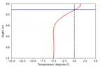
Soil temperature profile
Stand alone module
Explore how temperature varies within a soil over the course of a day or year, as heat gets conducted upward and downward in the profile.
Stand alone module
Explore how temperature varies within a soil over the course of a day or year, as heat gets conducted upward and downward in the profile.
Duration:
1.0 hrs
Model used:
(self-contained)
1.0 hrs
Model used:
(self-contained)
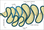
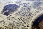
Meandering River Dynamics
Stand alone module
Meanderpy uses a simple linear relationship between the nominal migration rate and curvature, as recent work using time-lapse satellite imagery suggests that high curvatures result in high migration rates.
Stand alone module
Meanderpy uses a simple linear relationship between the nominal migration rate and curvature, as recent work using time-lapse satellite imagery suggests that high curvatures result in high migration rates.
Duration:
2.0 hrs
Model used:
Meanderpy
2.0 hrs
Model used:
Meanderpy
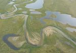
River-Delta Interactions
Stand alone module
Explore coastal processes by 1) a spreadsheet lab or 2) an advanced modeling lab using the CEM model. We look at the effects of waves and river avulsion on a coastline.
Stand alone module
Explore coastal processes by 1) a spreadsheet lab or 2) an advanced modeling lab using the CEM model. We look at the effects of waves and river avulsion on a coastline.
Duration:
1.5 hrs
Model used:
CEM
1.5 hrs
Model used:
CEM
CSDMS Workbench: Python Modeling Toolkit (pymt)
Stand alone module
The Python Modeling Toolkit (pymt) provides the tools needed for coupling models that expose a Basic Model Interface (BMI). This lab illustrates how to use pymt to run and couple models.
Stand alone module
The Python Modeling Toolkit (pymt) provides the tools needed for coupling models that expose a Basic Model Interface (BMI). This lab illustrates how to use pymt to run and couple models.
Duration:
2.0 hrs
Model used:
CEM
2.0 hrs
Model used:
CEM
Sediment Supply to the Global Ocean
Stand alone module
Investigate river sediment supply to the ocean by exploring the effects of climate changes on river fluxes. Also look at the effect of humans on rivers: the building of a reservoir.
Stand alone module
Investigate river sediment supply to the ocean by exploring the effects of climate changes on river fluxes. Also look at the effect of humans on rivers: the building of a reservoir.
Duration:
2.0 hrs
Model used:
HydroTrend
2.0 hrs
Model used:
HydroTrend
CSDMS Workbench: Landlab
Stand alone module
Landlab is an open-source Python-language package for numerical modeling of Earth surface dynamics. This lab illustrates how to use different Landlab components for modeling.
Stand alone module
Landlab is an open-source Python-language package for numerical modeling of Earth surface dynamics. This lab illustrates how to use different Landlab components for modeling.
Duration:
1.0 hrs
Model used:
Landlab
1.0 hrs
Model used:
Landlab
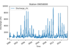
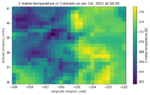
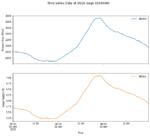
River Discharge Data Analysis
Stand alone module
Learn about river stage and discharge, using gage height data downloaded from the USGS for the upper Colorado River. Use standard Python libraries to read, analyze, and visualize data.
Stand alone module
Learn about river stage and discharge, using gage height data downloaded from the USGS for the upper Colorado River. Use standard Python libraries to read, analyze, and visualize data.
Duration:
3.0 hrs
Model used:
n/a
3.0 hrs
Model used:
n/a
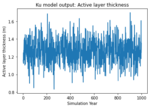
Permafrost Modeling with Ku Model
Stand alone module
This lab introduces how to use Ku model for permafrost modeling and how Ku can be used alongside landscape geomorphology models.
Stand alone module
This lab introduces how to use Ku model for permafrost modeling and how Ku can be used alongside landscape geomorphology models.
Duration:
1.5 hrs
Model used:
Kudryavtsev Model
1.5 hrs
Model used:
Kudryavtsev Model
Quantifying river channel evolution with Landlab
Stand alone module
This notebook illustrates the evolution of detachment-limited channels in an actively uplifting landscape.
Stand alone module
This notebook illustrates the evolution of detachment-limited channels in an actively uplifting landscape.
Duration:
2.0 hrs
Model used:
Landlab
2.0 hrs
Model used:
Landlab
SoilGrids Data Component
Stand alone module
A CSDMS data component used to download the soil property datasets from the SoilGrids system.
Stand alone module
A CSDMS data component used to download the soil property datasets from the SoilGrids system.
Duration:
1.0 hrs
Model used:
SoilGrids Data Component
1.0 hrs
Model used:
SoilGrids Data Component
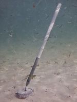
Tilt Current Meter Analyses
Stand alone module
Analyze month long deployment of velocity data from tilt current meters deployed in inlet stream in Maine
Stand alone module
Analyze month long deployment of velocity data from tilt current meters deployed in inlet stream in Maine
Duration:
2.0 hrs
Model used:
n/a
2.0 hrs
Model used:
n/a
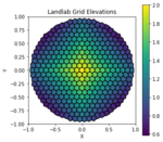
Alternative mesh generation for Landlab
Stand alone module
This lab uses the mesh generator dmsh and the mesh generator from the Anuga model to create unstructured grids that can be passed into Landlab.
Stand alone module
This lab uses the mesh generator dmsh and the mesh generator from the Anuga model to create unstructured grids that can be passed into Landlab.
Duration:
1.0 hrs
Model used:
Landlab
1.0 hrs
Model used:
Landlab
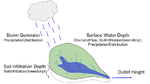
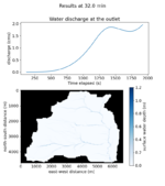
Exploring the effects of rainstorm sequences on a river hydrograph
Stand alone module
This notebook illustrates how storm sequences interact with watershed properties to control infiltration and runoff. It explores the relationships between rainfall intensity, water stage height, and infiltration through the integration of multiple Landlab components.
Stand alone module
This notebook illustrates how storm sequences interact with watershed properties to control infiltration and runoff. It explores the relationships between rainfall intensity, water stage height, and infiltration through the integration of multiple Landlab components.
Duration:
3.0 hrs
Model used:
Landlab
3.0 hrs
Model used:
Landlab
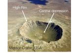
Cratered Landscapes
Stand alone module
Learn about the nature of impact craters and how we simulate their shape and distribution on a planetary surface. Then, investigate the results of different kinds of erosion on a cratered landscape, using Landlab.
Stand alone module
Learn about the nature of impact craters and how we simulate their shape and distribution on a planetary surface. Then, investigate the results of different kinds of erosion on a cratered landscape, using Landlab.
Duration:
1.5 hrs
Model used:
Landlab
1.5 hrs
Model used:
Landlab
GeoTiff Data Component
Stand alone module
Learn how to access data and metadata from a GeoTIFF file through an API or a BMI with the CSDMS GeoTiff Data Component.
Stand alone module
Learn how to access data and metadata from a GeoTIFF file through an API or a BMI with the CSDMS GeoTiff Data Component.
Duration:
1.0 hrs
Model used:
GeoTiff Data Component
1.0 hrs
Model used:
GeoTiff Data Component
Topography Data Component
Stand alone module
Learn how to download and access land elevation data from OpenTopography with the CSDMS Topography Data Component.
Stand alone module
Learn how to download and access land elevation data from OpenTopography with the CSDMS Topography Data Component.
Duration:
1.0 hrs
Model used:
Topography Data Component
1.0 hrs
Model used:
Topography Data Component
Including Wildfires in a Landscape Evolution Model
Stand alone module
Explore the effect of stochastic wildfires on riverine sediment flux. We use the SPACE model to simulate fluvial processes and introduce a stochastic wildfire model. Students can experiment by changing the rate of fires and other parameters.
Stand alone module
Explore the effect of stochastic wildfires on riverine sediment flux. We use the SPACE model to simulate fluvial processes and introduce a stochastic wildfire model. Students can experiment by changing the rate of fires and other parameters.
Duration:
1.0 hrs
Model used:
SPACE
1.0 hrs
Model used:
SPACE
Simulating Shoreline Change using Coupled Coastsat and Coastline Evolution Model (CEM)
Stand alone module
Visualize the evolution of any sandy beach in the world through time. learn how to extract complex datasets, run a geomorphic model, and explore the impact of different wave climates on a beach you care about.
Stand alone module
Visualize the evolution of any sandy beach in the world through time. learn how to extract complex datasets, run a geomorphic model, and explore the impact of different wave climates on a beach you care about.
Duration:
1.0 hrs
Model used:
CEM
1.0 hrs
Model used:
CEM
Linking Landlab Components and Creating Sediment Pulses in NetworkSedimentTransporter
Stand alone module
1) Demonstrate a potential to couple NST with existing landlab models that generate sediment sources or other sediment input condition; 2) Run the NetworkSedimentTransporter with pulses of sediment to understand the impact of landscape disturbance on sediment yield
Stand alone module
1) Demonstrate a potential to couple NST with existing landlab models that generate sediment sources or other sediment input condition; 2) Run the NetworkSedimentTransporter with pulses of sediment to understand the impact of landscape disturbance on sediment yield
Duration:
1.5 hrs
Model used:
River Network Bed-Material Sediment
1.5 hrs
Model used:
River Network Bed-Material Sediment
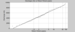
Flood Frequency Analyses with Python
Stand alone module
Analyze flood frequency of different rivers in North Carolina using basic extreme analysis and python. Students will get practice using pandas dataframes for importing, analyzing, and visualzing data.
Stand alone module
Analyze flood frequency of different rivers in North Carolina using basic extreme analysis and python. Students will get practice using pandas dataframes for importing, analyzing, and visualzing data.
Duration:
2.0 hrs
Model used:
n/a
2.0 hrs
Model used:
n/a
ERA5 Data Component
Stand alone module
A CSDMS Data Component used to access the ECMWF Reanalysis v5 (ERA5) climate datasets.
Stand alone module
A CSDMS Data Component used to access the ECMWF Reanalysis v5 (ERA5) climate datasets.
Duration:
1.0 hrs
Model used:
ERA5 Data Component
1.0 hrs
Model used:
ERA5 Data Component
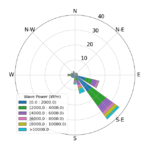
Data Component Use Case for Wave Power Calculation
Stand alone module
A demonstration of using the WAVEWATCH III Data Component to download wave properties datasets to calculate the wave power.
Stand alone module
A demonstration of using the WAVEWATCH III Data Component to download wave properties datasets to calculate the wave power.
Duration:
1.5 hrs
Model used:
WAVEWATCH III ^TM
1.5 hrs
Model used:
WAVEWATCH III ^TM

dbSEABED Data Component
Stand alone module
A CSDMS Data Component used to download the marine substrates datasets from the dbSEABED system.
Stand alone module
A CSDMS Data Component used to download the marine substrates datasets from the dbSEABED system.
Duration:
1.0 hrs
Model used:
dbSEABED Data Component
1.0 hrs
Model used:
dbSEABED Data Component

Topography to GRASS GIS to Landlab model grid
Stand alone module
A demonstration of fetching elevation data with the Topography data component, reprojecting and tuning it with GRASS GIS, then loading it into a Landlab RasterModelGrid.
Stand alone module
A demonstration of fetching elevation data with the Topography data component, reprojecting and tuning it with GRASS GIS, then loading it into a Landlab RasterModelGrid.
Duration:
1.0 hrs
Model used:
GRASS GIS, Landlab, Topography Data Component
1.0 hrs
Model used:
GRASS GIS, Landlab, Topography Data Component
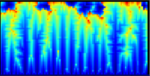
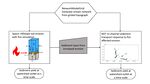
Data Component Use Case for Permafrost Thaw and Hillslope Diffusion
Stand alone module
A demonstration of how to use the Data Components, Landlab, and Pymt Model Components to simulate the permafrost active layer thickness and the hillslope diffusion process.
Stand alone module
A demonstration of how to use the Data Components, Landlab, and Pymt Model Components to simulate the permafrost active layer thickness and the hillslope diffusion process.
Duration:
1.5 hrs
Model used:
Kudryavtsev Model
1.5 hrs
Model used:
Kudryavtsev Model
Data Component Use Case for Overland Flow Simulation
Stand alone module
A demonstration of how to use the Data Components and Landlab components for overland flow simulation.
Stand alone module
A demonstration of how to use the Data Components and Landlab components for overland flow simulation.
Duration:
1.5 hrs
Model used:
Landlab
1.5 hrs
Model used:
Landlab
Data Component Use Case for Landslide Susceptibility Calculation
Stand alone module
A demonstration of how to use the Data Components to download topography and soil datasets to calculate the landslide susceptibility.
Stand alone module
A demonstration of how to use the Data Components to download topography and soil datasets to calculate the landslide susceptibility.
Duration:
1.5 hrs
Model used:
Landlab
1.5 hrs
Model used:
Landlab
NWIS Data Component
Stand alone module
A CSDMS Data Component designed to access USGS National Water Information System (NWIS) data.
Stand alone module
A CSDMS Data Component designed to access USGS National Water Information System (NWIS) data.
Duration:
1.0 hrs
Model used:
NWIS Data Component
1.0 hrs
Model used:
NWIS Data Component
Permafrost Modeling - where does permafrost occur?
Module 1 of 4 of the series Permafrost.
What is permafrost and how do you make a first-order prediction about permafrost occurrence. This is lesson 1 in a mini-course on permafrost, this lab uses the Air Frost Number and annual temperature data to predict permafrost occurrence.
Module 1 of 4 of the series Permafrost.
What is permafrost and how do you make a first-order prediction about permafrost occurrence. This is lesson 1 in a mini-course on permafrost, this lab uses the Air Frost Number and annual temperature data to predict permafrost occurrence.
Duration:
1.5 hrs
Model used:
Frost Model
1.5 hrs
Model used:
Frost Model
Permafrost Modeling - the Active Layer
Module 2 of 4 of the series Permafrost.
Explore what is active layer depth and the effects of snow and soil water content on permafrost. This is lesson 2 in a mini-course on permafrost. It employs a 1D configuration of the Kudryavtsev model.
Module 2 of 4 of the series Permafrost.
Explore what is active layer depth and the effects of snow and soil water content on permafrost. This is lesson 2 in a mini-course on permafrost. It employs a 1D configuration of the Kudryavtsev model.
Duration:
1.5 hrs
Model used:
Kudryavtsev Model
1.5 hrs
Model used:
Kudryavtsev Model
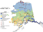
Permafrost Modeling - making maps from gridded climate data
Module 3 of 4 of the series Permafrost.
Using the Frost number code and grids of climate input data, one can make predictions of permafrost occurrence over the last century in Alaska. This is lesson 3 in a mini-course on permafrost.
Module 3 of 4 of the series Permafrost.
Using the Frost number code and grids of climate input data, one can make predictions of permafrost occurrence over the last century in Alaska. This is lesson 3 in a mini-course on permafrost.
Duration:
2.0 hrs
Model used:
Frost Model
2.0 hrs
Model used:
Frost Model
Permafrost Modeling - looking at future permafrost with climate models
Module 4 of 4 of the series Permafrost.
Using the Frost number code and grids of climate model input data (CMIP5), allows you to map predictions of permafrost occurrence. This is lesson 4 in a mini-course on permafrost.
Module 4 of 4 of the series Permafrost.
Using the Frost number code and grids of climate model input data (CMIP5), allows you to map predictions of permafrost occurrence. This is lesson 4 in a mini-course on permafrost.
Duration:
1.5 hrs
Model used:
Frost Model
1.5 hrs
Model used:
Frost Model
More labs: Archived labs
