Lab-0003
Permafrost Modeling - making maps from gridded climate data
This lab is part of the series Permafrost. Others in this series are:
- Permafrost Modeling - where does permafrost occur? (1 of 4)
- Permafrost Modeling - the Active Layer (2 of 4)
- Permafrost Modeling - making maps from gridded climate data (3 of 4)
- Permafrost Modeling - looking at future permafrost with climate models (4 of 4)
Contributor(s)
Classroom organization
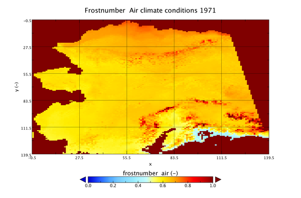
This lab is the third in a series of introduction to permafrost process modeling. In this third lesson, we further use the Air Frost number model and learn to use this model to create spatially varying predictions of permafrost in the CSDMS Python Modeling Tool (Pymt). We implemented the Air Frost number model (as formulated in Nelson and Outcalt, 1987). This pseudo-2D implementation is named the Frost-number GEO model.
This series of labs is designed for inexperienced modelers to gain some experience with running a numerical model, changing model inputs, and analyzing model output. Specifically, this lab combines the simple model with a climate reanalysis dataset, modified from the CRU-NCEP climate data over the 20th century. Basic information on the CRU_AK data component is presented in these slides. File:FrostNumberGEOModel Lecture3.pptx
This lab will likely take 1.5 -2 hrs to complete in the classroom. This time assumes you now have gained some familiarity with the Pymt and have learned how to set parameters, save runs, download data and look at output. If this is not the case, either start with Lab 1 in this series, or learn how to use Pymt (https://pymt.readthedocs.io/en/latest/install.html).
If you are a faculty at an academic institution, it is possible to work with us to get temporary teaching accounts. Work directly with us by emailing: csdms@colorado.eduDownload associated file: FrostNumberGEOModel Lecture3.pptx
Basic information on the CRU_AK data component is presented in these slides
Skills
- familiarize with a basic configuration of the Air Frost number Model for a gridded region.
- hands-on experience with visualizing NetCDF time series with Panoply.
- data to model comparisons and how to think about uncertainty in data and model output.
- what is a climate reanalysis product, what uncertainties does it have?
- what are regional differences in permafrost occurrence
- what are important parameters for assessing the state of permafrost in the future?
Lab notes
You can launch binder to directly run the Jupyter Notebook for this lab through a web browser.
>> Open a new browser window and open the Pymt read the docs page (https://pymt.readthedocs.io/en/latest/examples.html)
>> You will see that there are several example models.
>> Click on the 'Launch Binder' box and it will allow you to see this lab as a Jupyter Notebook.
>> You can execute the Jupyter notebook code cells using shift -enter.Requirements
--
Acknowledgements
These labs are developed with support from NSF Grant 1503559, ‘Towards a Tiered Permafrost Modeling Cyberinfrastructure’
References
- Nelson, F.E., Outcalt, S.I., 1987. A computational method for prediction and prediction and regionalization of permafrost. Arct. Alp. Res. 19, 279–288.
- Daly, C., et al., 2008. Physiographic sensitive mapping of climatological temperature and precipitation across the conterminous US. Int. J. Climatol. DOI: 10.1002/joc.1688
- Harris, I., Jones, P, Osborne, T, Lister, D., 2014. Updated high-resolution grids of monthly climaticobservations – the CRU TS3.10 Dataset. J. Climatol. 34: 623–642.
- Chadburn, S.E., Burke, E.J., Cox, P.M., Friedlingstein, P., Hugelius, G., Westerman, S., 2017. An observation-based constraint on permafrost loss as a function of global warming.Nature Climate Change, 10 APRIL 2017. DOI: 10.1038/NCLIMATE3262


