WMT tutorial
The CSDMS Web Modeling Tool (WMT) is the web-based successor to the desktop CSDMS Modeling Tool. WMT allows users to build and run coupled surface dynamics models on a high-performance computing cluster (HPCC) from a web browser on a desktop, laptop or tablet computer. You wil need an account on the CSDMS HPC Blanca, and this takes 3 business days to set up, apply here. If you are a faculty and want to use WMT for teaching a class, CSDMS and CU research computing can work with you to set up temporary teaching logins for multiple students.
This article gives a short tutorial on how to use WMT. For details on the buttonology of WMT, please see WMT Help.
Open WMT
In a web browser, go to
to open WMT.
Sign in
Sign in to WMT with an email and a password.
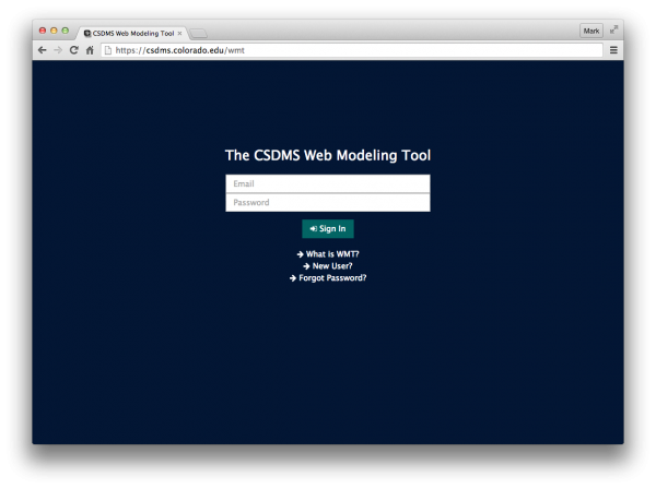
You have to be signed in to create, save and run models. If this is the first time you're signing in to WMT, you'll be prompted to repeat your password. Once you've signed in, you'll see the WMT interface:
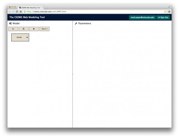
Select a driver for the model
To create a new model in WMT, you must start by selecting a component to act as the driver of the model.
In the Model panel, click the driver button and choose HydroTrend from the list of components displayed.
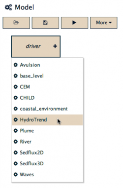
This adds HydroTrend as the driver of the model, as the Model panel now shows.
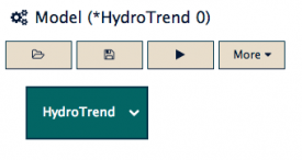
WMT has also given a generic Model title to the new model, based on the name of the driver component. We'll chose a more specific title when we save the model.
Get information on a model component
The HydroTrend model component you just added now acts as a button. Clicking it displays a new menu with a set of actions that can be performed on the model component.
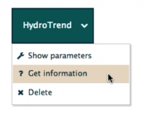
Let's choose to Get information on HydroTrend. Selecting this menu item displays a pop-up window giving the component name, version, DOI, a brief summary of its functionality, a link to the component's help page, and the author of the component.
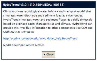
For detailed infomation, you can follow the link to the component help page on the CSDMS web site.
Edit a component parameter
When HydroTrend was selected, its parameters were displayed in the Parameter panel.
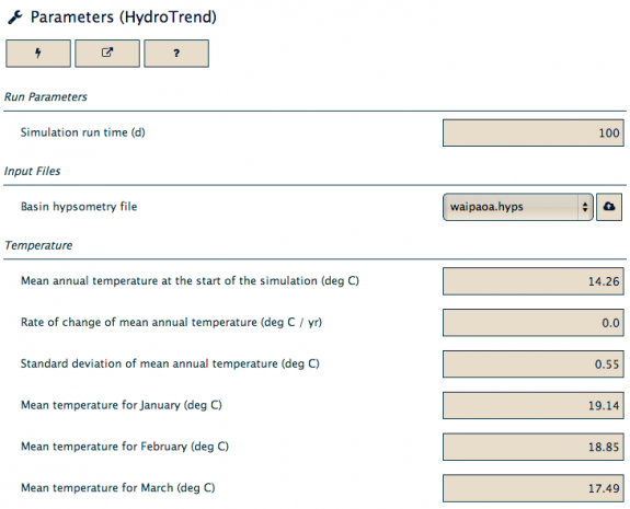
Each parameter used by HydroTrend is listed with a reasonable default value chosen by the developer. Try hovering over the first parameter, Simulation run time.

In addition to the default value, note that each parameter displays its range of possible values as a tooltip.
Each parameter is also editable.
Change the Simulation run time parameter from 100 to 365 days by entering the value 365 in the parameter's value box and selecting the <Enter> key.
Note that you can use scientific notation: 365 could be entered as 3.65E2.
[1]
If an out-of-range value is entered for a parameter, the value box turns red.

A model can still be saved and executed with out-of-range parameters present, but the results may be invalid. For this tutorial, use an in-range value of 365 days.
Add labels to the model
Model labels are used to group and categorize models in WMT. Attaching labels to a model can make it easier to find the model at a later time.
Open the Manage labels menu under the ![]() More... button in the Model panel.
Here you'll see a list of all public labels, shared among the community, as well as the private labels that belong only to you.
You'll see that a public label for HydroTrend (as the driver) has already been selected for this model.
More... button in the Model panel.
Here you'll see a list of all public labels, shared among the community, as well as the private labels that belong only to you.
You'll see that a public label for HydroTrend (as the driver) has already been selected for this model.
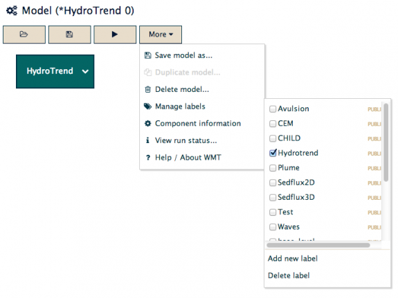
We can also add our own private labels. Let's add another private label, such as example or tutorial, to the model. Select the Add new label button on the labels menu (see figure above), and add the label of your choice. The menu will automatically update with the new label. Select the label ("checking" it) to attach it to the model.
Save the model
We're now ready to save the model.
Select the ![]() Save button in the Model panel.
You'll be presented with a dialog.
This is where you can change the name of the model, as well as review the labels attached to the model.
[2]
Save button in the Model panel.
You'll be presented with a dialog.
This is where you can change the name of the model, as well as review the labels attached to the model.
[2]
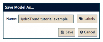
Note that the model is saved at CSDMS, not locally on your computer. Therefore, anywhere that you can access WMT, you can access your saved models. For example, you could design a model at your office, save it, and open it again on your home computer to edit it.
Run the model
To run the model, select the ![]() Run button in the Model panel.
You're presented with a dialog that allows you to choose the HPCC on which the model is run,
as well as your login credentials for that HPCC.
Currently, as of May 2018, CSDMS has setup its resources on Blanca. The HPCC nodes we use in tutorials are referenced as tlogin1.rc.colorado.edu or tutorial-login.rc.colorado.edu
If you don't already have an account on Blanca,
please visit the HPC accounts page to apply for a login.
Note that your login credentials for Blanca may not be the same as your WMT sign in!
Run button in the Model panel.
You're presented with a dialog that allows you to choose the HPCC on which the model is run,
as well as your login credentials for that HPCC.
Currently, as of May 2018, CSDMS has setup its resources on Blanca. The HPCC nodes we use in tutorials are referenced as tlogin1.rc.colorado.edu or tutorial-login.rc.colorado.edu
If you don't already have an account on Blanca,
please visit the HPC accounts page to apply for a login.
Note that your login credentials for Blanca may not be the same as your WMT sign in!
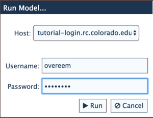
On a successful login, WMT submits the model run as a job on the HPCC, and you're presented with a status dialog.
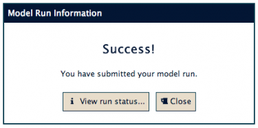
Clicking on the View run status... button takes you to the WMT Simulation Status page, where you can check on the status of your model run[3] and, when finished, download the results.

Examine the model output
Let's download the model output and examine the result.
The output is packaged as a *.tar.gz file.
Extract the contents using the tar shell command:
$ tar -zxf da2c78a3-0a4f-4beb-b053-80f9cb7738c0.tar.gz
$ cd da2c78a3-0a4f-4beb-b053-80f9cb7738c0/
$ ls -F
README           components.yaml  hydrotrend/      model.yaml
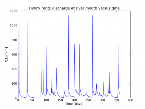
Let's make a simple plot of discharge versus time using Python.
After browsing the hydrotrend/ directory in the output, as well as consulting the Model:HydroTrend and Model_help:HydroTrend pages, the files we need are
- ./hydrotrend/HYDRO_OUTPUT/HYDROASCII.Q
for the discharge at the river mouth [m3s-1], and
- ./hydrotrend/_time.txt
for the model time steps [days].
In Python, start with the module imports.
We'll need numpy and matplotlib.
import matplotlib.pyplot as plt
import numpy as np
Next, read the time variable from its file.
with open("./hydrotrend/_time.txt", "r") as f:
    stime = f.read().split("\n")
Pop off the last two values from the list read from the file, then convert the data into a numpy array of type double.
stime.pop()
stime.pop()
time = np.array(stime)
Now read the discharge data.
with open("./hydrotrend/HYDRO_OUTPUT/HYDROASCII.Q", "r") as f:
    sdischarge = f.read().split("\n")
Remove the last value and the two header lines from the list read from the file before converting it into an array.
sdischarge.pop()
sdischarge.pop(0)
sdischarge.pop(0)
discharge = np.array(sdischarge)
Finally, visualize the model output as a time series with matplotlib.
plt.plot(time, discharge)
plt.title("HydroTrend: discharge at river mouth versus time")
plt.xlabel("Time [days]")
plt.ylabel("Q [$m^3 s^{-1}$]")
plt.show()
