Model:Sedflux

sedflux

sedflux-2.0

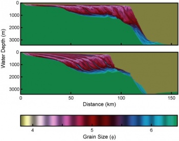
Sedflux-2.0 is the newest version of the Sedflux basin-filling model. Sedflux-2.0 provides a framework within which individual process-response models of disparate time and space resolutions communicate with one another to deliver multi grain sized sediment load across a continental margin. Version 2.0 introduces a series of new process models, and the ability to operate in one of two modes to track the evolution of stratigraphy in either two or three dimensions. Additions to the 2D-mode include the addition of models that simulate

1. erosion and deposition of sediment along a riverbed,
2. cross-shore transport due to ocean waves, and
3. turbidity currents and hyperpycnal flows.

New processes in the 3D-mode include

1. river channel avulsion,
2. two-dimensional diffusion due to ocean storms, and
3. two-dimensional flexure due to sediment loading.

The spatial resolution of the architecture is typically 1-25 cm in the vertical, and 10-100 m in the horizontal when operating in 2D-mode. In 3D-mode, the horizontal resolution usually extends to kilometers. In addition to fixed time steps (from days to hundreds of years), Sedflux-2.0 offers event-based time stepping as a way to conduct long-term simulations while still modeling low-frequency but high-energy events.

Introduction

Sedflux 2.0 is the newest version of the Sedflux basin-filling model. Sedflux 2.0 provides a framework within which individual process-response models of disparate time and space resolutions communicate with one another to deliver multigrain-sized sediment load across a continental margin. Version 2.0 introduces a series of new process models, and the ability to operate in one of two modes to track the evolution of stratigraphy in either two or three dimensions. Additions to the 2D mode include the addition of models that simulate (1) erosion and deposition of sediment along a riverbed, (2) cross-shore transport due to ocean waves, and (3) turbidity currents and hyperpycnal flows. New processes in the 3D mode include (1) river channel avulsion, (2) two-dimensional diffusion due to ocean storms, and (3) two-dimensional flexure due to sediment loading. The spatial resolution of the architecture is typically 1–25 cm in the vertical and 10–100m in the horizontal when operating in 2D mode. In 3D mode, the horizontal resolution usually extends to kilometers. In addition to fixed time steps (from days to hundreds of years), Sedflux 2.0 offers event-based time stepping as a way to conduct long-term simulations while still modeling low-frequency but high-energy events.

History

SEDFLUX is a product by combining the DELTA model series (e.g. version 2: Syvitski and Daughney, 1992; version 6: Syvitski and Alcott, 1995b) with the GRAIN (e.g. version 2: Syvitski and Alcott, 1993) and FACIES (unpublished) model series. DELTA was a multi-process SSM first written in ANSI-standard FORTRAN in 1986. DELTA was not intended to simulate the internal deposit architecture, rather to examine the evolving seafloor properties (grain size, accumulation rates) at a few locations, and the evolving bathymetry. GRAIN simulated the deposition of sediment from surface plumes emanating from river mouths. GRAIN and FACIES, also written in ANSI-standard FORTRAN, provided more ways of studying the character of the evolving deposits, in terms of grain size and bulk density of deposits. FACIES could read in values from a river discharge simulator (RIVER3: Syvitski and Alcott, 1995a), but the RIVER model series was not designed to handle evolving discharge conditions from long-term climate trends.

In 1996, SEDFLUX combined DELTA and FACIES into a hybrid ANSI-standard C-FORTRAN model. Various subsequent versions utilized different or upgraded versions of independent basin-scale process models (INFLO1: a hyperpycnal - turbidity current model: Skene et al., 1998; PLUME1.1: an advection-diffusion hypopycnal plume model: Syvitski et al., 1998a; BING: a visco-plastic debris flow model developed by G. Parker: Pratson et al., in press). SEDFLUX was also designed to read the output of the latest version of HYDROTREND (Syvitski et al., 1998b), a fully integrated river basin model that included the ability to simulate river mouth dynamics from climate-driven hydrology.

To provide for a much higher-resolution simulator (MOBIL Technology support) and seafloor characterizer (ONR support), SEDFLUX was recently (1999) rewritten in ANSI-standard C so that memory could be dynamically allocated during model runs. Since the publication of Syvitski and Hutton (2001), Sedflux has advanced along three major paths. The first is the addition of process models that operate solely within the 2D mode of Sedflux. The second is the expansion of the Sedflux architecture to be able to track stratigraphy in three dimensions and the addition of processes necessary to do this. The third are additions that operate in both the 2D and 3D mode.

Sedflux 2.0 (Hutton and Syvitski 2008) is a three-dimensional basin-filling model that is able to predict stratigraphy that varies laterally and vertically. The 3D mode of Sedflux records sediment deposition in two lateral dimensions while the 2D mode tracks sediment only in the cross-shore direction. The individual processes that operate within either mode of the Sedflux framework are either one- or two-dimensional. These processes produce sediment deposits that vary laterally (in either one or two dimensions) but use vertically averaged variables that only vary horizontally. The absence of three-dimensional models within Sedflux is not due to a limitation of its architecture but rather because these models are not yet incorporated.

Papers

1. Syvitski, J.P.M. 1989. The process-response model in Quantitative Dynamic Stratigraphy. In: T.A. Cross (ed.) Quantitative Dynamic Stratigraphy. Prentice-Hall, N.Y., p. 309-334.

2. Syvitski, J.P.M. and Andrews, J.T. 1994. Climate Change: Numerical modeling of sedimentation and coastal processes, Eastern Canadian Arctic. Arctic and Alpine Research, 26(3): 199-212.

3. Syvitski, J.P.M., Nicholson, M., and Skene, K., Morehead, M.D.1998. PLUME1.1: Deposition of sediment from a fluvial plume. Computers and Geoscience, 24(2): 159-171.

4. Syvitski, J.P.M. and Daughney, S. 1992. DELTA-2: Delta progradation and basin filling. Computers and Geosciences 18(7): 839-897.

5. Syvitski, J.P.M. and Alcott, J.M. 1993. GRAIN2: Predictions of particle size seaward of river mouths. Computers and Geoscience 19(3): 399 - 446.

6. Syvitski, J.P., and Hutton, E.H., 2001. 2D SEDFLUX 1.0C: An advanced process-response numerical model for the fill of marine sedimentary basins. Computers and Geoscience 27(6): 731-754.

7. Morehead, M.D., and Syvitski, J.P., 1999. River Plume Sedimentation Modeling for Sequence Stratigraphy: Application to the Eel Shelf, California. Marine Geology 154:29-41.

8. Syvitski, J.P.M., Pratson, L. O’Grady, D. 1999. Stratigraphic Predictions of Continental Margins for the Navy. In: J.W. Harbaugh, L.W. Whatney, E. Rankay, R. Slingerland, R. Goldstein, and E. Franseen (eds.) Numerical Experiments in Stratigraphy: Recent Advances in Stratigraphic and Computer Simulations. SEPM special publication. No. 62, 219-236.

9. Syvitski, J.P.M., and Bahr, D.B., 2001. Numerical Models of Marine Sediment Transport and Deposition. Computers and Geosciences, 27(6): 617-753.

10. Hutton, E.W.H. and Syvitski, J.P.M. 2004. Advances in the Numerical Modeling of Sediment Failure During the Development of a Continental Margin. Marine Geology, 203: 367-380.

11. Ross, W. C., Halliwell, B. A., May, J. A., Watts, D. E., and Syvitski, J. P. M. 1994. The Slope Readjustment Model: A New Model for the Development of Submarine Fan/Apron Deposits. Geology: 22: 511-514.

12. Syvitski, J.P.M. and Alcott, J.M. 1995. DELTA6: Numerical simulation of basin sedimentation affected by slope failure and debris flow runout. In: Pierre Beghin International Workshop on Rapid Gravitational Mass Movements, Grenoble, France, p. 305-312.

13. Mulder, T., Savoye, B. and Syvitski, J.P.M. 1997. Numerical modelling of the sediment budget for a mid-sized gravity flow: the 1979 Nice turbidity current. Sedimentology, 44: 305-326.

14. Skene, K., Mulder, T., and Syvitski, J.P.M. 1997. INFLO1: A model predicting the behaviour of turbidity currents generated at a river mouth. Computers and Geoscience, 23(9): 975-991.

15. Mulder T., Savoye B., Syvitski, J.P.M. and Piper, D.J.W. 1998. The Var Submarine Sedimentary System: understanding Holocene sediment delivery processes and their importance to the geological record. In M. S. Stoker, D. Evans, A. Cramp (editors): Geological Processes on Continental Margins: Sedimentation, Mass Wasting and Stability, Geol. Society, Spec. Publ., London, 145-166.

16. Mulder, T., Syvitski, J.P.M. and Skene, K. 1998. Modeling of erosion and deposition by sediment gravity flows generated at river mouths. Journal of Sedimentary Research, 67(3): 124-137.

17. Syvitski, J.P.M., Nicholson, M., and Skene, K., Morehead, M.D.1998. PLUME1.1: Deposition of sediment from a fluvial plume. Computers and Geoscience, 24(2): 159-171.

18. Skene, K., Piper, D.J.W., Aksu, A.E., and Syvitski, J.P.M. 1998. Evaluation of the global oxygen isotope curve as a proxy for Quaternary sea level by modeling of delta progradation. Journal of Sedimentary Research, 68: 1077-1092.

19. Syvitski, J.P.M., Pratson, L. O’Grady, D. 1999. Stratigraphic Predictions of Continental Margins for the Navy. In: J.W. Harbaugh, L.W. Whatney, E. Rankay, R. Slingerland, R. Goldstein, and E. Franseen (eds.) Numerical Experiments in Stratigraphy: Recent Advances in Stratigraphic and Computer Simulations. SEPM special publication. No. 62., 219-236.

20. Pratson, L., J. Imran, G. Parker, J.P.M. Syvitski & E.W.H. Hutton 2000. Debris flow versus turbidity currents: A modeling comparison of their dynamics and deposits. In: A.H. Bouma and C.G. Stone (eds.) Fine-Grained Turbidite Systems, 57-71. AAPG Memoir 72 and SEPM Special Publication No. 68, Tulsa, Oklahoma.

21. Bahr, D.B., Hutton, E.W.H., Syvitski, J.P., and Pratson, L., 2001. Exponential approximation to compacted sediment porosity profiles. Computers & Geosciences, 27(6): 691-700.

22. Morehead, M., Syvitski, J.P., and Hutton, E.W.H., 2001. The link between abrupt climate change and basin stratigraphy: A numerical approach. Global and Planetary Science, v. 28: 107-127.

23. O’Grady, D.B., and Syvitski, J.P.M., 2001. Predicting profile geometry of continental slopes with a multiprocess sedimentation model. In: D.F. Merriam and J.C. Davis (eds.) Geological Modeling and Simulation: Sedimentary Systems. Kluwer Academic/Plenum Publishers, New York, p. 99-117.

24. Pratson, L., Imran, J., Hutton, E., Parker, G., Syvitski, J.P., 2001. BANG1D: A one-dimensional, Lagrangian model of turbidity current mechanics. Computers and Geosciences, 27(6): 701-716.

25. Lee, H.J., Syvitski, J.P.M., Parker, G. Orange, D., Locat, J., Hutton, E.W.H. and Imran, J., 2002. Distinguishing sediment waves from slope failure deposits: Field examples, including the ‘Humboldt slide’, and modeling results. Marine Geology, 192: 79-104.

26. Syvitski, J.P.M. and Hutton, E.W.H., 2003. Failure of marine deposits and their redistribution by sediment gravity flows. Pure and Applied Geophysics. 160: 2053-2069.

27. Morehead, M.D., Syvitski, J.P.M., Hutton, E.W.H., and Peckham, S.D. 2003. Modeling the inter-annual and intra-annual variability in the flux of sediment in ungauged river basins. Global and Planetary Change. 39 (1/2): 95-110.

28. Kubo, Y., Syvitski, J.P.M., Hutton, E.W.H., Paola, C. 2005, Advance and application of the stratigraphic simulation model 2D-SedFlux: From tank experiment to geological scale simulation. Sedimentary Geology 178: 187-195.

29. Overeem, I., Syvitski, J.P.M., and Hutton, E.W.H., 2005, Three-dimensional numerical modeling of deltas. In: L. Giosan and J.P. Bhattacharya (Eds.) River Deltas — Concepts, Models, and Examples. SEPM Special Publication No. 83, pp. 13-30.

30. Overeem, I., Syvitski, J.P.M., Hutton, E.W.H., and Kettner, A.J. 2005. Stratigraphic variability due to uncertainty in model boundary conditions: a case-study of the New Jersey Shelf over the last 21,000 years. Marine Geology 224: 23-41.

31. Syvitski, J.P.M., Pratson, L.F., Wiberg, P.L., Steckler, M.S., Garcia, M.H., Geyer, W.R., Harris, C.K., Hutton, E.W.H., Imran, J., Lee, H.J., Morehead, M.D., and Parker, G., 2007. Prediction of margin stratigraphy. In: C.A. Nittrouer, J.A. Austin, M.E. Field, J.H. Kravitz, J.P.M. Syvitski, and P.L. Wiberg (Eds.) Continental-Margin Sedimentation: From Sediment Transport to Sequence Stratigraphy. IAS Spec. Publ. No. 37: 459-530.

32. Parsons, J. Friedrichs, C., Garcia, M., Imran, J., Mohrig, D., Parker, G., Pratson, L., Puig, P., Syvitski, J.P.M., Traykovski, P. 2007. Sediment gravity flows: Initiation, transport and deposition. In: C.A. Nittrouer, J.A. Austin, M.E. Field, J.H. Kravitz, J.P.M. Syvitski, and P.L. Wiberg (Eds.) Continental-Margin Sedimentation: From Sediment Transport to Sequence Stratigraphy. IAS Spec. Publ. No. 37: 275-338.

33. Kraft, B.J., Overeem, I., Holland, C.W., Pratson, L.F., Syvitski, J.P.M., and Mayer, L.M., 2006, Stratigraphic model predictions of geoacoustic properties. IEEE Journal of Ocean Engineering, 31(2): 266-283.

34. Pratson, L.F., Hutton, E.W.H. Hutton, A.J. Kettner, J.P.M. Syvitski, P.S. Hill, Douglas A.G., T.G. Milligan, 2007, The Impact of floods and storms on the acoustic reflectivity of the inner continental shelf: A modeling assessment. Continental Shelf Research, 27: 542–559.

35. Kubo, Y., Syvitski, J.P.M., Hutton, E.W.H., Kettner, A.J. 2006, Inverse modeling of post Last Glacial Maximum transgressive sedimentation using 2D-SedFlux: Application to the northern Adriatic Sea. Marine Geology 234: 233-243.

36. Hutton E.W.H., and Syvitski, J.P.M., 2008, SedFlux2.0: An advanced process-response model that generates three-dimensional stratigraphy. Computers & Geosciences, 34: 1319-1337.

37. Jouet, G, Hutton, E.W.H., Syvitski, J.P.M., Rabineau, M., Berné, S. 2008, Modeling the isostatic effects of sealevel fluctuations on the Gulf of Lions. Computers & Geosciences, 34: 1338-1357.

38. Kettner A.J., B. Gomez, E.W.H. Hutton and J.P.M. Syvitski, 2008, Late Holocene dispersal and accumulation of terrigenous sediment on Poverty Shelf, New Zealand, Basin Research 21(2): 253-267

sedflux Questionnaire

Contact Information

Model	sedflux
Contact Person	Eric Hutton
Institution	University of Colorado
City	Boulder, CO
Country	USA
Email:	--
2nd person involved:	--
3rd person involved:	--

Model Description

Model type:	Modular model
Description:	Sedflux-2.0 is the newest version of the Sedflux basin-filling model. Sedflux-2.0 provides a framework within which individual process-response models of disparate time and space resolutions communicate with one another to deliver multi grain sized sediment load across a continental margin.

Technical Information

Supported platforms:	Unix, Linux, Mac OSX
Programming language:	C
Model was developed started from:	1997 and development still takes place
To what degree will the model become available:	As code and as executable
Current license type:	GPL_v2
Memory requirements:	2GB
Typical run time:	minutes to days

Input / Output Description

Input parameters:	River mouth characteristics (velocity, width, depth, concentration) averaged daily, or longer. Initial bathymetry. Input sediment distribution and properties of each grain type. Optionally, any of: tectonics, sea level, wave climate, and currents
Input format:	ASCII
Output parameters:	Sediment properties that include (but are not limited to) bulk density, grain size, porosity, and permeability. These are averaged over are user-specified vertical resolution (typically mm to cm). Sea-floor properties that include slope, water depth, and sand fraction.
Output format:	Binary
Post-processing software (if needed):	no
Visualization software (if needed):	Yes, Matlab

Process Description

Processes represented by model:	surface plumes, hyperpycnal plumes, sediment slope failure that results in turbidity currents or debris flows, subsidence, compaction, sediment remobilization due to waves and currents, river avulsion
Key physical parameters & equations:	Too numerous to list.
Length scale & resolution constraints:	Vertically: mm to cm; Horizontally: 10s of m to 1000 of m
Time scale & resolution constraints:	Days or greater. Component processes can have much higher resolutions for numerical stability.
Numerical limitations and issues :	--

Testing

Available calibration data sets:	--
Available test data sets:	--
Ideal data for testing:	--

User Groups

Currently or plans for collaborating with:

None

Documentation

Key papers of the model:	Hutton and Syvitski, 2008 (doi:10.1016/j.cageo.2008.02.013) Syvitski and Hutton, 2001 (doi:10.1016/S0098-3004(00)00139-4)
Is there a manual available:	Yes
Model website if any:	http://sedflux.googlecode.com

Additional Comments

Comments:

No

Issues

To report an issue with sedflux, please go to its development site on googlecode: http://code.google.com/p/sedflux/issues/list

Help

SubversionSedflux

Checkout a version of sedflux

Checkout a version

To checkout the latest version of sedflux

svn checkout (https://instaar.colorado.edu/svn/Main/sedflux)

The code is in sedflux/trunk.

svn status

svn diff

svn commit

sedfluxRiverFile

Description of a sedflux river file

The river file specifies river characteristics of the river as it enters the model domain. It can come in two formats: key-value file (ASCII), or Hydrotrend (binary). Regardless of format, the river format specifies river width, depth, velocity, and concentrations of each of the grain types. In both cases, if sedflux runs through all of the periods of your river file, it will return to the beginning.

Key-value File

The user can specify river characteristics key-value pairs for an arbitrary number of time periods. Unlike the Hydrotrend file, these time periods need not be the same length. The following example defines two periods,

[ 'Season 1' ] Duration (y): 3m Bedload (kg/s): 300.0 Suspended load concentration (kg/m^3): 6, 3, 3, 3 velocity (m/s): 1.0 Width (m): 100.0 Depth (m): 5.0 [ 'Season 2' ] Duration (y): 9m Bedload (kg/s): 30.0 Suspended load concentration (kg/m^3): .6, .3, .3, .3 velocity (m/s): 1.0 Width (m): 10.0 Depth (m): .5

The first period lasts for 3 months, and the second for 9 months (the periods need not sum to 1 year - they can be whatever length you like).

Note

The durations that you specify in this file will override the time step that you provided in the initialization file. Thus, say you provided a time step of 1 day in the initialization file. If using the above river file, this time step would be ignored and would instead alternate between 3 months and 9 months.

Hydrotrend File

The Hydrotrend model can output daily, monthly, or yearly river data. See the Hydrotrend web page for a detailed description of the format. One thing to note though is that it is binary and will be of the byte-order of the machine that it was created on. It has been a common problem for users to use a Hydrotrend file created on one machine but then run sedflux with this file on a machine with the opposite byte-order. sedflux should now be able to notice this and give an appropriate error message

SedfluxSubsidenceFile

Description of a sedflux subsidence file sedflux Subsidence file

The format for sedflux subsidence files is different for the 2D and 3D versions of sedflux. In 2D mode, the subsidence file is a series of records that each contain a time value, and comma delimated data that define the subsidence curve. In 3D mode, the subsidence file is also a series of records that defines a time-varying subsidence curve but is binary.

2D subsidence file

The subsidence file in the following example contains two records that define the subsidence of the profile at 0 and 100 years. Each record begins with a header contained in square brackets followed by two columns of data that define how the profile subsides along its length. The time is given in years, the position (first column) in meters, and the subsidence rate (second column) in meters per year. For times between records, sedflux interpolates linearly between records.

[ Time: 0 ] // Time of this record in years 0, 0 // Subsidence is zero at the origin 100000, -.2 // and increases to -.2 m/y at 100km

[ Time: 100 ] // The second record is at 100 years 0,0 100000, -.1

If the file contains only one record, then the subsidence rate is held constant starting from the time indicated in the record header. If the model runs longer than the time of the last record, the subsidence curve is set to that of the last record for the remainder of the simulation.

3D subsidence file

The subsidence file for 3D sedflux, contains a series of binary records containing similar information as that of the 2D file described above.

The file begins with two 32-bit integers that define the size of the subsidence grid for each record. The first value is the number of rows and the second the number of columns.

Records are then listed one after another. Each record begins with a double value that gives the time in years of the record. The subsidence data then follows as double values written row by row. Subsidence values are given in meters per year.

Note

The size of the grid must match exactly that of the grid that is defined in the bathymetery file.

Note

The byte order of the file must be the same as that of the machine that the simulation will be run on.

SedfluxSeaLevelFile

Description of a sedflux sea-level file sedflux Sea-Level File

A sedflux sea-level file consists of two comma-separated columns that specify sea-level with time. The first column is time (in years), and the second is elevation (in meters). sedflux uses linear interpolation to find sea-level between points. A simple sea-level file looks like this,

0 , 0 3000, -10 6000, 5

Here sea level falls 10 meters over 3000 years, and then rises 15 meters over the next 3000 years.

SedfluxBathymetryFile

Description of a sedflux Bathymetry file sedflux bathymetry file

The initialization file lists the file that defines the initial bathymetry for a sedflux simulation. The format of the file depends on whether sedflux will be run in 2D or 3D mode. In either case, though, all elevations are measured in meters.

2D mode

When run in 2D mode, sedflux only requires bathymetric elevations along a profile. This is provided as comma-separated columns with each row being a point along the profile. The first column is horizontal position of the point (in meters), and the second elevation (in meters). As an example:

0.00, 5.00 300.00, 3.00 500.00, 1.00 1329.4, -10.9 5200.0, -20.4 11282.4, -29.6 15540.0, -38.0 22894.1, -48.0 25890.0, -69.0 27317.6, -77.0 27732.4, -79.0 28976.5, -89.0 30082.4, -99.0 30911.8, -109.0 32017.6, -113.0

In this case the profile is just over 32 km long and drops 118 meters. The points need not be evenly spaced; sedflux will use linear interpolation to estimate elevations between points.

3D mode

The contents of the bathymetry is a matrix of elevations (in meters). Unlike the 2D version, sedflux does not interpolate between points. The points are spaced uniformly with the spacing specified by the x and y resolutions in the sedflux initialization file. As an example,

33,-8 ,-8.1 ,-8.2 ,-8.3 ,-8.4 ,-8.5 ,-8.6 ,-8.7 ,-8.8 33,-11 ,-11.1,-11.2,-11.3,-11.4,-11.5,-11.6,-11.7,-11.8 33,-13 ,-13.1,-13.2,-13.3,-13.4,-13.5,-13.6,-13.7,-13.8 33,-14 ,-14.1,-14.2,-14.3,-14.4,-14.5,-14.6,-14.7,-14.8 33,-14 ,-14.1,-14.2,-14.3,-14.4,-14.5,-14.6,-14.7,-14.8 33,-14.5,-14.6,-14.7,-14.8,-14.9,-15 ,-15.1,-15.2,-15.3 33,-14.7,-14.8,-14.9,-15 ,-15.1,-15.2,-15.3,-15.4,-15.5 33,-15 ,-15.1,-15.2,-15.3,-15.4,-15.5,-15.6,-15.7,-15.8 33,-15.2,-15.3,-15.4,-15.5,-15.6,-15.7,-15.8,-15.9,-16 33,-15.2,-15.3,-15.4,-15.5,-15.6,-15.7,-15.8,-15.9,-16

In this case, sedflux will use a 10 by 10 model grid. The spacing of the columns is the x-resolution and the spacing of the rows is the y-resolution.

InputFiles

List of input files for sedflux

Sedflux Input Files

The main input files are:

• Initialization file
• Bathymetry file
• Sediment description file
• Process definition file

The above are all required files. Files that are optionally included are:

• River file
• Sea-level file
• Subsidence file

Many of these files, are of a similar format (sedflux key-file).

SedfluxInitFile

Description of the sedflux initialization file Initialization File

A sedflux initialization file is divided into two parts. The first part defines some global parameters while the second divides the model run into one or more "epochs". Each epoch defines a time step, duration, and process environment.

Global Parameters

The following is an example of a group that defines the global parameters for a sedflux simulation.

[ global ] margin name: poverty_bay vertical resolution: 0.05 x resolution: 30000 y resolution: 100 bathymetry file: poverty_bay_bathy.csv sediment file: poverty_bay_sediment.kvf

Each of these parameter/value pairs must be specified whether run in 2D or 3D mode. A brief description of the parameters: margin name The name of the sedflux simulation. This name will appear in the name of sedflux output files vertical resolution The vertical resolution (in meters) of the model run. Sediment deposits will be averaged over this amount. x resolution Resolution of the model run in the x-direction. For a 2D simulation this will be the along shore width over which sediment deposited. For 3D simulations, this refers to the spacing of rows in the bathymetry file. y resolution Resolution of the model run in the y-direction. For a 2D simulation this will be the resolution of the simulation in the cross-shore. For 3D simulations, this refers to the spacing of columns in the bathymetry file. bathymetry file The name of the file that specifies the initial bathymetry of the simulation. sediment file The name of the file that defines the type of sediment that is used by the model.

Epoch Parameters

The following is an example of a series of groups that define epoch parameters for a simulation.

[ epoch ] number: 1 duration: 490y time step: 1d process file: poverty_bay1.epoch

[ epoch ] number: 2 duration: 60y time step: 1d process file: poverty_bay2.epoch

[ epoch ] number: 3 duration: 300y time step: 1d process file: poverty_bay3.epoch

Here three epochs are specified. Each has its own duration and process file. Thus, in this example, the total simulation models 850 years. A brief description of the parameters, number Number that specifies the order that sedflux will run the epochs. sedflux runs epochs in ascending order. duration The length of the epoch ('y' for years, 'm' for months, and 'd' for days). time step The time step of the epoch ('y' for years, 'm' for months, and 'd' for days). IMPORTANT: Note that this parameter may be ignored (see NOTE at the bottom of this page). process file The name of the file that defines the processes for the epoch.

Note

If within the epoch process file the river values are specified as 'season', the time step given in that file will override that specified in the initialization file.

RunningSedflux

Running sedflux

Running sedflux-2.0

Step 1: Setting up the input files

To run sedflux-2.0 you will need to create a project directory where the input files will be stored and the output files can be written to. You will need at least four input files. Depending on the processes that you plan to use, you may need more (example input files are provided with the distribution within the share/sedflux_input_files directory). these four files are,

• an initialization file
• a sediment file
• a bathymetry file
• a process file

Initialization file

The initialization file will usually end with a .init extension. the name of this file can be passed to sedflux on the command line:

sedflux --init-file=<init-file>

where <init-file> is the name of the initialization file. in this case, the project directory is the current working directory. if you do not specify any command line arguments, you will be prompted to give a project directory and the name of the initialization file. Note

This syntax was introduced in version 2.0.8. Previous versions used

sedflux in=<init-file> \endcode

Note

Windows note: most likely you will not be using command line arguments and so will have to enter the project directory and initialization file by hand. in this case, to specify a directory on another filesystem, begin the path with the drive letter followed by a colon. as an example,

c:/My Sedflux Projects/This project

Make sure to use forward slashes (/) rather than back slashes (\).

Sediment file

The sediment file specifies a number of grain types that will be used to fill the basin. each grain type has a set of parameters that are specific to it. examples of grain type parameters are: grain size, grain density, saturated density, etc. any number greater than one grain type can be specified. the first grain type listed is interpreted by sedflux to be bed load. the rest of the grains are assumed to be suspended load. the particular name of the sediment file is specified within the init file.

Bathymetry file

The bathymetry file specifies the elevation of the initial floor of the model run. elevations can be thought to be given with respect to sea level. negative elevations are below sea level. the data is contained within an ascii file as in two comma-separated columns. note however, that the data must be preceded by a line that indicates the start of the data as such,

0, 10 40000, -200 100000, -200

each column is in meters. sedflux interpolates between these points to match the resolution of the model run. the name of the bathymetry file is provided in the init file. sedflux 3D Note

If run in 3d mode, the format of the bathymetry file is different. Instead of two columns of data, the file contains a grid of comma-separated values that indicate bathymetric elevation in meters. Each row represents elevation values of constant y-positions. The spacing of the points is specified in the initialization file as x-resolution and y-resolution.

Process file

This is the largest of the input files. You use this file to control the various processes that sedflux will model. Each process begins with a line of the form:

[ <process-name> ]

where <process-name> is the name of a particular process ('sea level', or erosion, for example). This is then followed by four label/value pairs. They will look something like:

process name: sea level active: yes logging: no repeat interval: always

The meaning of each of the labels are:

• process name

The name of the process. It does not have to match the name in the preceding line. It is only used for writing to log files and for debugging.

• active

should sedflux model this process or not? if 'yes', sedflux will run the specified process. if 'no', the process will be skipped.

• logging

if 'yes' additional information will be written to a log file as well as to the screen. this information is really only of interest for debugging purposes.

• repeat interval

specify how often the process will be run. some processes may operate on longer time scales then others and so may not need to be run as frequently as others. this value can either be the keyword 'always', or a period of time. 'always' indicates that the process should be run with every time step. a duration is given as a series of numbers followed by a time unit (d=day, m=month, y=year). as an example: 1y is yearly, 7d is weekly, 1y 6m is 1.5 yearly etc. if this duration is less than the time step of the run (as provided in the init file), it is set to this time step and so is run with every time step.

Subsequent label/value pairs within a process are specific to each process. I hope that the labels by themselves are sufficient as a description. Unfortunately, i'm sure this is not always the case.

Step 2: Running sedflux

To run sedflux,

> cd <project-dir> > sedflux --init-file=<init-file>

where <project-dir> is the directory where you set up you input files, and <init-file> is the name of your initialization file. sedflux 3D Note

By default, sedflux will run in 2D mode. To run sedflux in 3D mode, use the '-3' option,

> sedflux -3 --init-file=<init-file>

Step 3: Reading the output files

A small library of MATLAB mfiles is included with the sedflux-2.0 distribution that read plot the various output files. When you installed sedflux, they were put into the directory <sedflux-prefix>/share/ew. You can either copy these files into you MATLAB directory, or add this path to in your startup.m file.

There are two types of output files for sedflux-2.0: property files, and measuring station files. The output of both of these file types is done in the process file. For property files, this is done in the group called data dump. For example,

[ 'data dump' ] process name: data dump active: yes logging: yes repeat interval: 1000y output directory: ./output-grain vertical resolution: full horizontal resolution: full vertical limits: tight horizontal limits: tight property: grain

In this case, sedflux will write a property file of average grain size every 1000 years. The process specific key/value pairs are:

• output_directory

The directory (relative to the root directory for the simulation) where sedflux will write this output file.

• vertical_resolution

The vertical resolution of the output file. 'full' indicates the resolution of the simulation. This parameter is ignored in the current version. 'full' is assumed.

• horizontal resolution

The horizontal resolution of the output file. 'full' indicates the resolution of the simulation. This parameter is ignored in the current version. 'full' is assumed.

• vertical_limits

The minimum and maximum limits of the vertical extent of the output. 'tight' indicates that the limits will be those of the simulation. This parameter is ignored in the current version. 'tight' is assumed.

• horizontal_limits

The minimum and maximum limits of the vertical extent of the output. 'tight' indicates that the limits will be those of the simulation. This parameter is ignored in the current version. 'tight' is assumed.

• property

A key that indicates what sediment property sedflux will output.

In this example, sedflux will write a series of files (to the directory \p output-grain) of the form, <simulation-name>####.grain. Where <simulation-name> is the name of the simulation as specified in the initialization file, and #### is a four digit number. For each successive file written, the number is incremented by 1 (starting at 0001).

The second type of output file is a measuring station file. Again, you can control the output of this file from the process file through the 'measuring station' group. For example,

[ 'measuring station' ] process name: measuring station active: yes logging: yes repeat interval: always parameter to measure: depth position wrt river mouth: no position of station: all filename: ./output/test.depth

Here, sedflux flux will write depth information every time step (as specified with the 'always' key).

The process-specific parameters are:

• parameter to measure

A key that indicates what parameter sedflux should measure.

• wrt to river mouth

Should horizontal positions be measured with respect to the river mouth or as absolute distances. This should be either 'yes' or 'no'.

• position of station

The location of the measuring stations. 'all' indicates that a measuring station be positioned at every position within the simulation This is disabled in the current version. 'all' is assumed.

• filename

The filename of the output file.

Unlike the property file process that writes a series of files, sedflux creates only one measuring station file for every measured parameter.

The MATLAB function used to plot a property file is plot_property. If we have called our simulation 'My_Simulation', we might use the following to look at some output,

>> plot_property( 'My_Simulation0001.grain' )

To read the data from a measuring station file, use the command read_measuring_station_cube,

>> [z,x,t,h]=read_measuring_station_cube( 'test.depth' );

Here, z will be a matrix that contains all of the measurements, x is the positions of the measuring stations, t is an array of times the measurements were made, and h contains some header information from the file. To plot up this output, simply use the plot command,

>> plot( x(2,:,1) , z(:,1,[1 end] )

In this case we have potted the first and last sets of measurements.

ConfiguringSedflux

Configuring the sedflux build directory Configuring

The configure command

To configure sedflux-2.0:

> configure --prefix=<program-prefix>

where <program-prefix> is the path name to the location into which the program will be install. For example, <program-prefix> could be /usr/local/sedflux. In this case, all of the sedflux installation files will be installed in /usr/local/sedflux. This would mean that the sedflux executable program would be /usr/local/sedflux/bin/sedflux.

Configuration options

--enable-libgtk

If you have gtk+-2.0 (version >= 2.2) installed on you machine you can compile the graphical user interface for sedflux. The default is to disable this functionality. If enabled, configure will search for the libraries using pkg-config. (http://www.gtk.org)

--enable-libcheck

If you have check package installed, you can compile sedflux to include unit tests. The default is for unit tests to be disabled. If enabled, configure will use pkg-config to find the required libraries and header files. (http://check.sourceforge.net)

--enable-doxygen

Generate HTML documentation. This must be done using the program doxygen. If enabled, doxygen must be in your PATH. The default is to disable doxygen. (http://www.stack.nl/~dimitri/doxygen)

--enable-blas --with-blas-dir=PATH

Currently, there is only minimal support for BLAS/LAPACK libraries. If you wish to use these libraries rather than the ones that come with the distribution, you can indicate such with the --enable-blas option. If pkg-config can not find the necessaty libraries, you can manually specify the base path of the BLAS installation with the --with-blas-dir=PATH option.

--with-html-dir=PATH

Specify a location to put HTML documentation. If not specified, documentation is installed in ${datadir}/ew-doc/html.

Troubleshooting

Problem

I get an error message saying that I don't have gtk+-2.0 (or glib) but I know I do.

Solution

The configure script uses pkg-config to find the required libraries. Make sure that you have set your PKG_CONFIG_PATH environment variable to include the pkg-config files for these libraries. As an example,

> setenv PKG_CONFIG_PATH /usr/local/lib/pkgconfig

Problem

PKG_CONFIG_PATH is set correctly but configure still says that my version of glib is not correct.

Solution

Locate the path to the library files for your latest version of glib-2.0. Make sure that this path is listed before (or at all) the older library files in your LD_LIBRARY_PATH environment variable. To check the contents of LD_LIBRARY_PATH,

> echo $LD_LIBRARY_PATH

If the glib libraries (libglib-2.0.so, libgthread-2.0.so, etc.) are in /usr/local/lib, you can set LD_LIBRARY_PATH as,

> setenv LD_LIBRARY_PATH /usr/local/lib:$LD_LIBRARY_PATH

Problem

configure finds the correct version of glib but reports an error when trying to link to it.

Solution

You probably need to add some library directories to you LD_LIBRARY_PATH environment variable. Open config.log and search for the error. There will be a record of the error that the compiler encountered. If it is something like 'library not found for -lintl', make sure that if the intl library is not in a standard location, that it is in your LD_LIBRARY_PATH. For instance,

> setenv LD_LIBRARY_PATH /usr/local/gnu/lib

SedfluxModBioturbation

Description of the bioturbation module

Introduction

sedflux implements one of two bioturbation modules. The first is diffusion-based while the second is a biological 'conveyor-belt'. Both models are described in Boudreau, 1997.

Boudreau, B.P., 1997, Diagenetic Models and Their Implementation: Modelling Trasport and reactions in Aquatic Sediments: Berlin, Springer-Verlag, 414 pp.

Bioturbation as diffusion

The sediment column is divided into a series of layers. Organisms in the sediment are assumed to move sediment randomly either up or down. This results in the reworking of sediment being a diffusive process. Thus, for some sediment layer,

dui / dt = d ( K dui / dz ) / dz

where t is time, z is burial depth, K is the biological diffusion coefficient, and ui is the amount of sediment from the i-th layer. This processes is carried out for each sediment layer within some burial depth. Typically, this depth is around 10cm. Measured biological diffusion coefficients range from 10-100 cm^2/year.

Bioturbation as a conveyor belt

In the conveyor-belt model, organisms move sediment from some depth and deposit it on the sea floor. Such a model is known as a non-local model as sediment jumps from one location to another. The current implementation of this model assumes a constant burial depth from which sediment is moved from and that it is transported at a constant rate, R. Thus, over a period of Dt, this process will mix an amount of sediment given by,

Dh = R Dt

Typically, R is given in units of cm/day and is on the order of 1.

Example

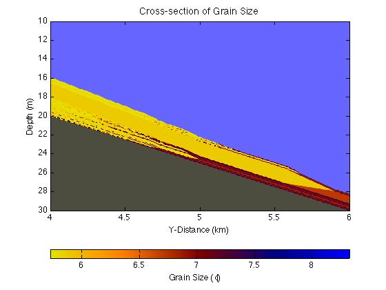
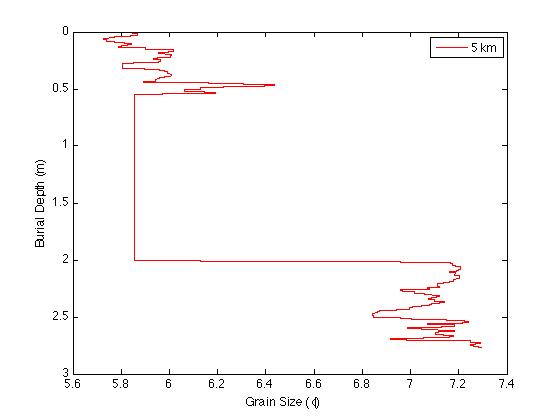
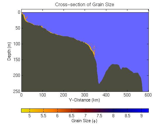
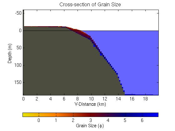
As a control, we deposit 20 years worth of sediment using a simulated daily time series of sediment discharge from the Eel River, California. The initial bathymetry is a linear slope that approximates the Eel River shelf. We then run the same simulation with the only difference being that bioturbation (diffusion) turned on (K=50cm^2/y). The following figures compare the grain-size profiles for the control (left figure) and diffusion (right figure) experiment.

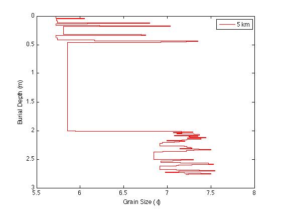
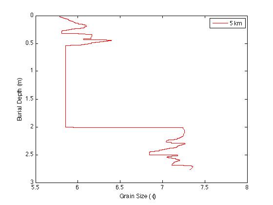
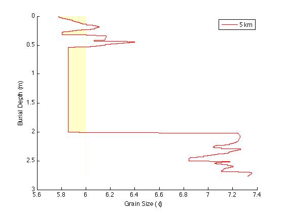
For further comparison, the following figures show grain size cores taken at y=5km for the same two simulations.

VisualizingSedflux

Visualizing sedflux output with MATLAB

There are two main sedflux output files: the property file and the measuring station file. Both are binary files that can be read and visualized through MATLAB.

Reading and visualizing a property file

The plot_property and read_property MATLAB functions are used to visualize and read data from a sedflux property file, respectively.

plot_property

The MATLAB function used to plot a property file is plot_property. The same function is used for output generated with sedflux run in either 2D or 3D mode. However, some of the options vary defending on the mode.

plot_property for 2D mode

For our first example, we consided a property file of average grain size that was generated by sedflux run in 2D-mode. For the simulation called, 'sedflux_2D_simulation', we can use the following to look at some output,

>> plot_property( 'sedflux_2D_Simulation0001.grain' );

If all goes well, MATLAB should generate an image of the average grain size over the profile.

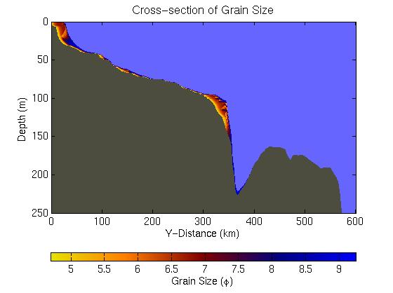
Following the name of the file, the user can specify a series of parameter/value pairs that control how the image is displayed. For instance, the following parameter/value pairs print the time (in years), scale the data between 2 and 10 (phe units), and remove the colorbar.

>> plot_property( 'sedflux_2D_Simulation0001.grain' , 'time' , 21000 , 'clim' , [2 10] , 'colorbar' , false );

Other parameters are 'func', and 'mask'. Use func to specify a function handle that will operate on the property data. The function should take a matrix as its only input parameter. Continuing with the previous example, we can plot grain size in millimeters rather than phe units using the func parameter.

>> plot_property( 'sedflux_2D_Simulation0001.grain' , 'func' , @(f)(2.^(-f)) );

A data mask is a matrix of logical values that is the same size as the data to be plotted. To create a mask, one usually reads in the data and then creates the mask based on those data values. This requires the MATLAB function read_property (explained later). In the following example, we wish to only plot those data between 2 and 6 phe units.

>> [f,h] = read_property( 'sedflux_2D_Simulation0001.grain' ); >> plot_property( 'sedflux_2D_Simulation0001.grain' , 'mask' , f>2 & f<6 );

plot_property for 3D mode

The following MATLAB command plots a slice of sedflux 3D cube. In this example we plot a slice of grain size along the plane at x=3.2km. One can also specify a slice of constant y or z (use 'yslice' or 'zslice', respectively).

>> plot_property( 'sedflux_3D_Simulation0001.grain' , 'xslice' , 3.2 );

plot_property_core

To plot a core from a property file, use plot_property_core. The following plots a grain-size core at position y=5km,

>> plot_property_core( 'Bioturbation0019.grain' , 5 )

and produces the following,

Optional parameter/value pairs are:

• overlay Overlay the core plot over a property file image
• burial Use burial depth (m) for the vertical axis rather than elevation
• time Specify a property file of age to convert burial depth to age
• sand Specify a phe value for sand. Grain sizes coarser than this will be filled with yellow.

read_property

Need to add something here.

Reading and visualizing a measuring station file

To create a surface plot from a measuring station file use plot_measuring_station_surface. The following command plots the last record from a sedflux measuring station file of bathymetric elevation.

>> plot_measuring_station_surface( 'KL-elevation.bin' , 'zdir' , 'norm' ) >> set( gca , 'dataaspectratio' , [1 1 20] )

The 'zdir' parameter is set to 'norm' to ensure the data are plotted right-side up. The aspect ratio is changed to better visualize the surface.

CompilingSedflux

Compiling and installing sedflux

Step 1: Install prerequisites

Before attempting to compile sedflux make sure that you have all of the prerequisite packages. You may not need the particular versions; those are only the versions that I use.

Step 2: configure the distribution

Run the configure script provided with the distribution. Note that if you have changed any Makefile.am or configure.in files, you may have to run the bootstrap command that is provided with distribution.

Step 3: compile and install sedflux

A description of how the build and install sedflux is provided here.

SedfluxPrerequisites

Prerequisites need to compile sedflux

Prerequisites

To install sedflux-2.0, you need to have certain progams installed on you machine. A list of these programs follows with the version numbers that I used. It is possible that older version will work but I have not checked if this is the case.

Required

• pkg-config (0.21)
• automake (1.9.6)
• autoconf (2.61)
• gcc (2.95.3)
• glib-2.0 (2.12.12)
• libtool (1.5.24)

Optional

• (http://check.sourceforge.net/) check(0.9.4)
• (http://www.stack.nl/~dimitri/doxygen/) doxygen(1.5.1)
• (http://www.gtk.org/) gtk+-2.0(2.2.4)

If you do not have some of the optional programs, you can still install sedflux but with some loss of functionality. The limitations are:

• check: You will not be able to run unit tests on your compiled code.
• doxygen: You will not be able to generate documentation
• gtk+-2.0: You will not be able to run the graphical user interface

The configure script will check for these packages and turn them on or off depending are whether or not they are found.

BuildingSedflux

Build and install sedflux

Build

To compile the sedflux-2.0 package,

> make

Once this has finished, you can install the package,

> make install

This will copy all of the sedflux installation files to the location you specified during the configuration process. Note that you will have to have write permission for the directory that you are installing into.

Building for 64 bit Machines

This really just describes how I go about building a 64-bit version of sedflux on our Solaris machines.

All it takes is to define correctly the necessary environment variables. To make sure we use the proper compiler and linker, set the environment variables CC and \LD. For our machine this means,

> setenv CC /usr/local/lang/bin/cc > setenv LD /usr/ccs/bin/sparcv9/ld

Now set CFLAGS to compile the 64 bit code,

> setenv CFLAGS "-xarch=v9b -xCC"

Optionally, to build faster running code I'll instead use,

> setenv CFLAGS "-fast -xarch=v9b -xCC -xautopar -xO5"

To make sure the correct libraries are linked to, I'll define \p LDFLAGS as,

> setenv LDFLAGS "-L/usr/lib/sparcv9 -L/usr/ucblib/sparcv9 -L/usr/local/sparcv9/lib"

The sedlux configure script uses pkg-config to locate required libraries (usually, this is just glib-2.0). To make sure that it finds the 64-bit versions, set your PKG_CONFIG_PATH to include these paths. For our system, this is

> setenv PKG_CONFIG_PATH /usr/local/sparcv9/lib/pkgconfig

Finally, because I'm paranoid, I'll remove all references to the regular 32 bit libraries from my LD_LIBRARY_PATH. Somehow, no matter how hard I try, LD tries to link to these libraries instead of the 64 bit versions.

SedfluxSedimentFile

Description of the sedflux sediment file

Sediment File

The characteristics of each sediment type is defined by key-value pairs in its own group. A group begins with [ <group-name> ], is followed by a series of key-values pairs, and ends at the start of the next group (or EOF). The key-value lines are of the form:

<name-of-key> : <value>

Groups are listed one after another. The order that they occur here is important. sedflux assumes that the order they appear here corresponds to the same order as the river input files.

For a sediment file, the required parameters are: grain size Grain size (in microns) of the sediment type. grain density Density (in kg/m^3) of the sediment grains. saturated density Bulk density (in kg/m3) that the sediment saturated with water. minimum void ratio Void ratio (-) of the sediment in its closest packed state. diffusion coefficient Diffusion index between 0 (unable to be moved) and 1 (easily moved). removal rate Removal rate (in 1/day) consolidation coefficient How quickly the sediment consolidates. compaction coefficient Rate that sediment is compacted under load.

Note

The first grain type listed in the sediment file is assumed by sedflux to be bedload! That is, it is not carried by the plume process but by the bedload dumping process.

SedfluxKeyValueFile

Description of the sedflux key-value file

Many of the (ascii) input files for sedflux are of a common format. I'll often refer to them as sedflux key-files. They are plain text files that define a series of groups. Each group then contains a series of key-value pairs. A group begins with its name surrounded by braces and ends at the begining of the next group.

The key-value pairs then follow, one per line. They consist of a parameter name (or key), follows by a colon, and then the value. As an example, a valid group looks like,

[ global ] vertical resolution (m): 0.05 x resolution (m): 10000 y resolution (m): 100

In this example, we've defined a group called global. For this group, we've set the values for three parameters. There can be any number of groups or key-value pairs per file. In fact, the same group name can appear in the same file more than once. The data are not overwritten but a new instance of the group created. However, in some instances it may not make sense to have multiple occurances of a group.

Download

Source-Code Snapshots

Nightly Snapshot

The latest version of sedflux can be found on the CSDMS ftp site as sedflux-latest.tar.gz. This will always point to the latest version.

http://csdms.colorado.edu/pub/models/sedflux/sedflux-latest.tar.gz

Releases

No releases yet

Past Snapshots

sedflux-2.0.37.tar.gz (28/12/2007)

sedflux-2.0.34.tar.gz (21/12/2007)

Extras

Installer

sedflux-contractor-0.1.tar.gz

Input Files

sedflux-input-0.1.tar.gz

Regression Tests

sedflux-tests-0.1.tar.gz

Visualization Files

sedflux-mfiles-0.1.tar.gz

Source

To browse the sedflux repository, point your browser to: http://csdms.colorado.edu/viewvc/sedflux/?root=sedflux

Command-Line Access

If you plan to make changes, use this command to check out the code as yourself using HTTPS:

<geshi lang=bash>

1. Project members authenticate over HTTPS to allow committing changes.

svn checkout https://csdms.colorado.edu/svn/sedflux/sedflux </geshi>

When prompted, enter your CSDMS Subversion password.

Non-members may only check out a read-only working copy of the project source.

To obtain a CSDMS Subversion account or to become a member of this project, please email csdms@colorado.edu.

GUI and IDE Access

This project's Subversion repository may be accessed using many different client programs and plug-ins. See your client's documentation for more information.

Subversion Help

For help on how to use Subversion, an excellent manual is available online at http://svnbook.red-bean.com/