Labs PLUME

Plume Modeling

Once we have moved sediment and water over hillslopes and routed it through a river system, we can think about this flux of water and sediment draining into lakes or into the ocean. Typically the riverine freshwater and the suspended sediments will form a so-called hypopycnal sediment plume. We will use a component called PLUME to investigate the behavior of these sediment plumes. The model is largely based on turbulent jet theory presented by Albertson et al., (1950).
In this lab we will look at the river plume characteristics and the depositional patterns for single plume events.

STEP1 Load the PLUME component

>> Open the CMT, Go to Projects, Courses, choose 2013.
>> Drag the PLUME component into the driver palette.
>> Specify a unique working directory for each experiment, for example: /CMT_Output/PLUME1
>> (…etc PLUME2 for the next experiment).

River Characteristics
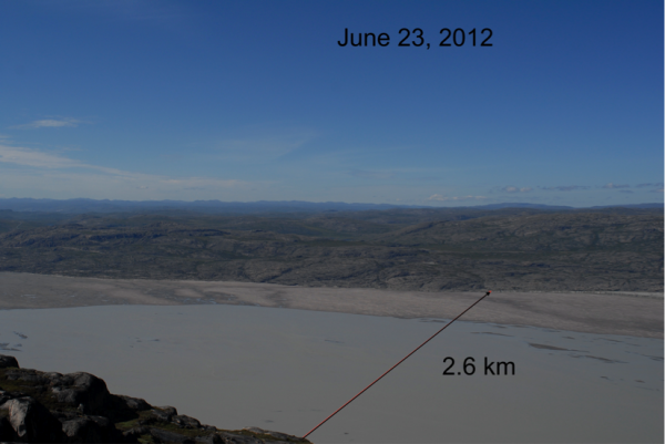
In this lab we will focus on a specific braided river system in West-Greenland. The Watson River drains a small section of the Greenland Ice Sheet, it winds through a narrow braided river plain for about 20km and then drains into Kangerlussuaq Fjord. The photo shows the river braidplain in 2012, which was a peak discharge year in Greenland The waterdepths on the braidplain are typically not very deep (>1m with perhaps a smaller channel section that is deeper ~ 3m).

Question 1
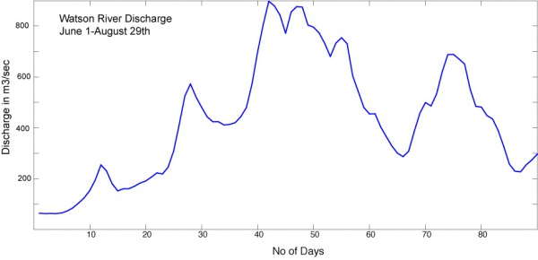
Use the annual hydrograph of the Watson River to estimate discharge events for 2 days in the summer. 
Indicate what your choosen dates and discharges are. The photo above will help to estimate a river mouth width. 
Can you estimate the river flow velocity? Please motivate your answer.

>> Set up two simulations of plume model for the different discharge events you have estimated. Keep each run at 10 days total simulation time, with each discharge event to last for 2 days and ask for an output grid for every 2 days. The default basin into which the river drains is a narrow fjord (2km wide by 30 km long), this can be changed to 4 km wide and 60km long to match the fjord dimensions of our case-study. Make sure you switch the output file ON!
>> You can use the ‘flood’ tab in the plume model to configure your simulations for the selected river input parameters. >> Once your simulation has completed, download the generated depositional grid for visualization in VisIT: ‘model_grain_class_0__deposition_rate.nc’

Question 2
How far out did sediment get deposited by the plume during early season conditions and how far out at high melt season conditions? 
How thick was the thickest deposit for each of the two events? Plot your two output grids.