Model:GIPL: Difference between revisions
m Text replace - "|Categories=" to "}} {{Model identity2 |Categories=" |
m Text replace - "|Categories=" to "}} {{Model identity2 |Categories=" |
||
| Line 1: | Line 1: | ||
{{Model identity | {{Model identity | ||
|Model type=Single | |Model type=Single | ||
}} | |||
{{Model identity2 | |||
}} | }} | ||
{{Model identity2 | {{Model identity2 | ||
Revision as of 09:58, 25 July 2011
GIPL
Metadata
|
|
|
Introduction
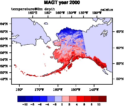
GIPL(Geophysical Institute Permafrost Laboratory) is an implicit finite difference one-dimensional heat flow numerical model. The model was developed by V.Romanovsky and G. Tipenko at University of Alaska Fairbanks. First time GIPL was introduced at the 2004 AGU Conference Tipenko G. (2004). The model uses coarse vertical resolution grid which preserves the latent-heat effects in the phase transition zone, even under conditions of rapid or abrupt changes in the temperature fields. It includes upper boundary condition (usually air temperature), constant geothermal heat flux at the lower boundary (typically from 500 to 1000 m) and initial temperature distribution with depth. The other inputs are precipitation, prescribed water content and thermal properties of the multilayered soil column. As an output the model produces temperature distributions at different depths, active layer thickness and calculates time of freeze up. S. Marchenko and others in 2008 extended the model by developing pre-processing procedures which convert GIS format input data into GIPL format. E. Jafarov parallelized the GIPL code in order to run the model on supercomputers with finer grid resolution. The first run of parallel UAF-GIPL2.0 model was in November 2009. The model is still under constant testing and development. However the preliminary results are available in the form of netcdf files. The preliminary results includes temperatures at different depths and active layer thickness. The detailed paper about the parallel model is under development.
IRF
The spatial model consist of three parts: pre-processing, GIPL run and post-processing.
As an input data for the model we use the SNAP(Scenarios Network Planning for Alaska) five GCM composite dataset with A1B emission scenario, which is available on-line and can be freely downloaded from the SNAP web-site.
Pre_processing includes processing of the SNAP dataset by converting it to GIPL input format. When the input dataset is ready we run the Message Passing Interface (MPI) parallel GIPL model. After GIPL run we post-process the model output by converting it netcdf univariate format, which then can by visualized with freely and commercially available softwares like ncview, IDV or ArcGIS.
Issues
Does not include convective heat transfer.
Visualization
References
Tipenko G, Marchenko S, Romanovsky S, Groshev V, Sazonova T. 2004. Spatially distributed model of permafrost dynamics in Alaska. Eos Transactions AGU, 85(47): Fall Meet. Suppl., Abstract C12A-02.
Marchenko SS, Romanovsky VE, Tipenko G. 2008. Numerical modeling of spatial permafrost dynamics in Alaska. In Proceedings of the Ninth International Conference on Permafrost, 29 June–3 July 2008, Fairbanks, Alaska. Institute of Northern Engineering, University of Alaska, Fairbanks.


