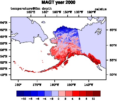
Model:GIPL: Difference between revisions
m Text replacement - "Add_model_references" to "Include_references_models_cargo" |
m Text replacement - "{{End headertab}}" to "{{End headertab}} {{{{PAGENAME}}_autokeywords}}" |
||
| (16 intermediate revisions by the same user not shown) | |||
| Line 5: | Line 5: | ||
{{End a table}} | {{End a table}} | ||
{{Model identity2 | {{Model identity2 | ||
| | |ModelDomain=Terrestrial, Cryosphere | ||
|Spatial dimensions=1D | |Spatial dimensions=1D | ||
|Spatialscale=Global, | |Spatialscale=Continental, Global, Landscape-Scale, Regional-Scale | ||
|One-line model description=GIPL(Geophysical Institute Permafrost Laboratory) is an implicit finite difference one-dimensional heat flow numerical model. | |One-line model description=GIPL(Geophysical Institute Permafrost Laboratory) is an implicit finite difference one-dimensional heat flow numerical model. | ||
|Extended model description=GIPL(Geophysical Institute Permafrost Laboratory) is an implicit finite difference one-dimensional heat flow numerical model. The GIPL model uses the effect of snow layer and subsurface soil thermal properties to simulate ground temperatures and active layer thickness (ALT) by solving the 1D heat diffusion equation with phase change. The phase change associated with freezing and thawing process occurs within a range of temperatures below 0 degree centigrade, and is represented by the unfrozen water curve (Romanovsky and Osterkamp 2000). The model employs finite difference numerical scheme over a specified domain. The soil column is divided into several layers, each with distinct thermo-physical properties. The GIPL model has been successfully used to map permafrost dynamics in Alaska and validated using ground temperature measurements in shallow boreholes across Alaska (Nicolsky et al. 2009, Jafarov et al. 2012, Jafarov et al. 2013, Jafarov et al. 2014). | |Extended model description=GIPL(Geophysical Institute Permafrost Laboratory) is an implicit finite difference one-dimensional heat flow numerical model. The GIPL model uses the effect of snow layer and subsurface soil thermal properties to simulate ground temperatures and active layer thickness (ALT) by solving the 1D heat diffusion equation with phase change. The phase change associated with freezing and thawing process occurs within a range of temperatures below 0 degree centigrade, and is represented by the unfrozen water curve (Romanovsky and Osterkamp 2000). The model employs finite difference numerical scheme over a specified domain. The soil column is divided into several layers, each with distinct thermo-physical properties. The GIPL model has been successfully used to map permafrost dynamics in Alaska and validated using ground temperature measurements in shallow boreholes across Alaska (Nicolsky et al. 2009, Jafarov et al. 2012, Jafarov et al. 2013, Jafarov et al. 2014). | ||
| Line 36: | Line 36: | ||
|Start year development=2000 | |Start year development=2000 | ||
|Does model development still take place?=Yes | |Does model development still take place?=Yes | ||
|DevelopmentCode=As is, no updates are provided | |||
|DevelopmentCodeYearChecked=2020 | |||
|Model availability=As code | |Model availability=As code | ||
|Source code availability=Through web repository | |Source code availability=Through web repository | ||
| Line 75: | Line 77: | ||
{{Additional comments model}} | {{Additional comments model}} | ||
{{CSDMS staff part | {{CSDMS staff part | ||
|OpenMI compliant= | |OpenMI compliant=No but possible | ||
|IRF interface= | |IRF interface=No but possible | ||
|CMT component=In progress | |CMT component=In progress | ||
|CCA component= | |PyMT component=Yes | ||
|CCA component=No but possible | |||
}} | }} | ||
{{DOI information | {{DOI information | ||
| Line 84: | Line 87: | ||
|DOI assigned to model version=0.1 | |DOI assigned to model version=0.1 | ||
|DOI-year assigned to model version=2011 | |DOI-year assigned to model version=2011 | ||
|DOI-filelink= | |DOI-filelink=https://csdms.colorado.edu/pub/models/doi-source-code/gipl-10.1594.IEDA.100131-0.1.tar.gz | ||
}} | }} | ||
{{Start coupled table}} | {{Start coupled table}} | ||
{{End a table}} | {{End a table}} | ||
{{End headertab}} | {{End headertab}} | ||
{{{{PAGENAME}}_autokeywords}} | |||
<!-- PLEASE USE THE "EDIT WITH FORM" BUTTON TO EDIT ABOVE CONTENTS; CONTINUE TO EDIT BELOW THIS LINE --> | <!-- PLEASE USE THE "EDIT WITH FORM" BUTTON TO EDIT ABOVE CONTENTS; CONTINUE TO EDIT BELOW THIS LINE --> | ||
| Line 106: | Line 111: | ||
== References == | == References == | ||
<br>{{ | <br>{{AddReferenceUploadButtons}}<br><br> | ||
{{#ifexist:Template:{{PAGENAME}}-citation-indices|{{{{PAGENAME}}-citation-indices}}|}}<br> | {{#ifexist:Template:{{PAGENAME}}-citation-indices|{{{{PAGENAME}}-citation-indices}}|}}<br> | ||
{{ | {{Include_featured_references_models_cargo}}<br> | ||
== Links == | == Links == | ||
Latest revision as of 19:17, 16 September 2020
GIPL
Metadata
|
|
|
Introduction
GIPL(Geophysical Institute Permafrost Laboratory) is an implicit finite difference one-dimensional heat flow numerical model.The model uses fine vertical resolution grid which preserves the latent-heat effects in the phase transition zone, even under conditions of rapid or abrupt changes in the temperature fields. It includes upper boundary condition (usually air temperature), constant geothermal heat flux at the lower boundary (typically from 500 to 1000 m) and initial temperature distribution with depth. The other inputs are precipitation, prescribed water content and thermal properties of the multilayered soil column. As an output the model produces temperature distributions at different depths, active layer thickness and calculates time of freeze up. The results include temperatures at different depths and active layer thickness, freeze-up days.
IRF
Issues
Does not include convective heat transfer.
Visualization
References
| Nr. of publications: | 30 |
| Total citations: | 1331 |
| h-index: | 17 |
| m-quotient: | 0.77 |
| Featured publication(s) | Year | Model described | Type of Reference | Citations |
|---|---|---|---|---|
|
Jafarov, E E; Romanovsky, V E; Genet, H; McGuire, A D; Marchenko, S S; 2013. The effects of fire on the thermal stability of permafrost in lowland and upland black spruce forests of interior Alaska in a changing climate. Environmental Research Letters, 8, 035030. 10.1088/1748-9326/8/3/035030 (View/edit entry) | 2013 | GIPL |
Model application | 122 |
|
Sazonova, T. S.; Romanovsky, V. E.; 2003. A model for regional-scale estimation of temporal and spatial variability of active layer thickness and mean annual ground temperatures. Permafrost and Periglacial Processes, 14, 125–139. 10.1002/ppp.449 (View/edit entry) | 2003 | GIPL Kudryavtsev Model |
Related theory | 114 |
| See more publications of GIPL |


