Labs WMT SEDFLUX2D
Modeling Stratigraphy in 2-D cross-sections
To learn more about Sedflux and its approach you can download this presentation.
For visualizations of the Sedflux output you can use free software VisIT, download the latest version here
STEP1 Load the 2D Sedflux component
>> If you have never used WMT, learn how to use it here.
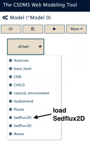
>> Pick SedFlux2D from the list of components in WMT
>> SedFlux2D component is the sole driver of this simulation, so there is no need to assemble its ports.
STEP 2 Building out a Delta into a Marine Basin
Assemble a SedFlux2D simulation to run a simple 2000 year simulation. Note that this means you will need to specify the run duration to be 730,000 days. We will simulate the evolution of a longitudinal profile of 100 km, with a shelf break at 50km and sloping to -250m at 100 km offshore; these are the default settings. The bathymetry tab allows us to set up a simple bathymetric profile. More complex bathymetry data can be loaded by using a *.csv file.
Let’s assume the receiving shelf width to be relatively narrow (25km). A relatively narrow basin reduces the available accommodation space and thus will speed up the vertical sedimentation rates (so there is more for us to see in the results).
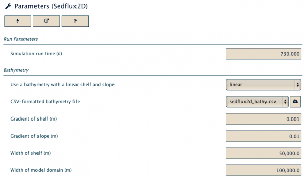
For this example simulation the sea level is stable at 0m (this happens when sea level is set to be to be 0m both at the beginning and end of the simulation ).
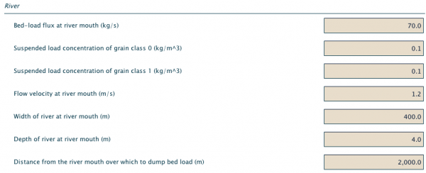
Our marine delta receives a constant river water flux of almost 2000 m3/s with 3 grainsizes traveling at capacity (bedload, and 2 classes of suspended load).
You can find these settings under the ‘sediment tab’, we will use the defaults.
>> Specify that you’d like 10 outputs: one for every 73,000 days (or 200 years).
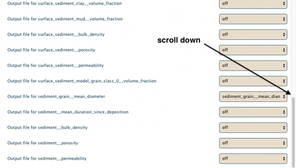
>> Request output of the entire stratigraphic cross section; the file is called 'sediment_grain_mean_diameter.nc'.
>> Note that this requires some scrolling-down to find this specific parameter. There are many other options for output.
>> Run this simulation.
>> You will be able to see progress of your run 'View Run Status’ window.
>> These simulations will take a little while (probably less than 10 minutes), refresh your browser to see the run-time ticking away
>> To get output from your run, transfer files from Beach to your local machine.
>> You now have the generated output file, called: ‘sediment_grain__mean_diameter.nc’
STEP3 Visualize a 2D Sedflux cross-section
>> Open‘sediment_grain__mean_diameter.nc’ file in VisIT
>> Use the pseudo-color plotting to draw the profile.
>> Under the ‘Plot Attributes’ tab in VisIT, set the limits to be 1 (minimum) and 8 (maximum).
>> To visualize the cross-section well you will need to apply two operators: CoordSwap and Transform.
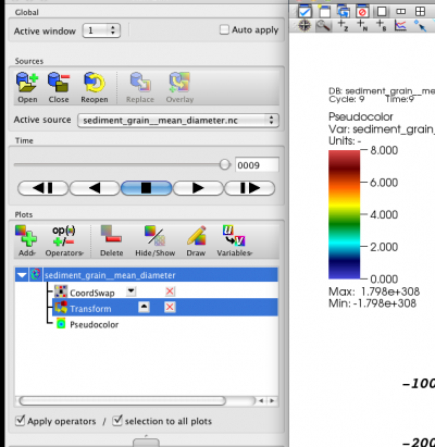
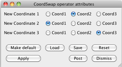
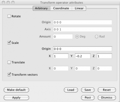
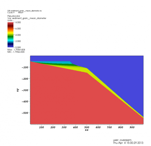
This basic run will have the following delta cross-section built up in 2000 years.
Question 1
What are the units in the legend? Please provide the conversion between the grainsize diameter in microns and the legend units.
Question 2
What do you see in this simple model experiment?
Is this typical delta stratigraphy? What is this pattern called?
Explore the active processes in this simple scenario
Models should not function as a ‘black box’. In the next section we look at your options to peak into the machinerie of Sedflux. The core of the Sedflux model consists of the plume model. There is another lab specially dedicated to the plume component
Question 3
Can you figure out from the parameter panel which processes are active and which processes are not in the default simulation?
Question 4
How is bedload distributed in Sedflux 2D, please list the equation.
What parameters influence this process?
Is the value set for ‘bedload dumping distance’ in the configuration realistic?
Sea Level Change Experiments
The key parameter that was historically called upon to explain stratigraphic patterns was sea level. Sea level explains a lot of longterm coastline shifting and specific patterns of progradation and retrogradation can be attributed to sea level change. In these exercises we will run a series of sea level scenarios: a rising sea level, a falling sea level and a full sea-level cycle.
Set up your initialization, these are the master parameters of the simulation. We’ll keep the duration short (3000 years) to keep the run-time manageable. Similarly the basin width is set to be 25km, and grid spacing 100m long by 0.1m thick.
We will create a number of sea level files to run: a rising sea level, a falling sea level and a sine-shaped (full cycle sealevel). These should just be *.csv files. A sea-level file for a falling sea level will specify run-time of 3,000 years and sealevel fall of 120 m over this timespan as two columns, as simple as this:
0, 0
3000, -120
You can create these files in a text editor, or Excel, save them as a*.csv format and then upload them to your specific directory on Beach. Subsequently you can use the ‘Sea Level’ tab to point to the file you want to be used for the simulation.

These runs will take ~ 20 minutes. In the meantime we will plot up the controlling input files to make an overview of sea level scenarios.
>> Plot the bathymetry and sealevel files as two panels.
Question 5
Formulate a ‘conceptual model’ for each of the scenarios.
Draw out what you expect to happen to the delta wedge stratigraphy.
You can try to do this for the shape of the depositional wedge as well as the grain-size trend.
Take into account the Sedflux is only running with 3 grain size classes for these experiments, which limits the complexity of your depositional package.
>> Now download the output files and plot 2D profiles for the different timeslices.
Question 6
What is the effect of a rapidly falling sea level on the stratigraphy?
What is the effect of a rising sea level?
What is the effect of a cosine-shaped sea level cycle?
Sea Level Change Experiments
Another major control on stratigraphy is ‘accommodation’. The space available for deposition, this is controlled by tectonics in the long-term. We will look at the control of accommodation on a much shorter time-scale, by looking at the effect of the initial bathymetric slope on the depositional package.
>> Construct two different bathymetry scenarios using the bathymetry parameters.
Use a stable sea level scenario, and run for 3000 years, this helps you explore the effect of the different initial profile conditions independent of the sea level fluctuation. These runs will take ~20 minutes. In the meantime we will plot up the controlling bathymetric files to see the initial profiles.
Question 6
You are now armed with more experience with simple Sedflux runs, formulate a ‘model’ for each of your bathymetry scenarios.
Draw out what you expect to happen to the stratigraphy.
You can try to do this for the shape of the depositional wedge as well as the grain-size trend.
Question 7
Once you have the output; what is the effect of slope on the stratigraphy? How fast does the coastline shift?
References
- Hutton, E. W. H. and Syvitski, J. P. M., 2008. Sedflux 2.0: An advanced process-response model that generates three-dimensional stratigraphy. Computer & Geosciences, 34, 1319~1337, Doi: (10.1016/j.cageo.2008.02.013).
- Syvitski, J. P. M. and Hutton, E. W. H., 2001. 2D SEDFLUX 1.0C: an advanced process-response numerical model for the fill of marine sedimentary basins. Computer & Geosciences, 27, 731~753, Doi: (10.1016/S0098-3004(00)00139-4).
