Labs WMT FuturePermafrost

Introduction to Permafrost Processes - Lesson 4 Explore the Future of Permafrost

This lab has been designed and developed by Irina Overeem and Mark Piper, CSDMS, University of Colorado, CO
with assistance of Kang Wang, Scott Stewart at CSDMS, University of Colorado, CO, and Elchin Jafarov, at Los Alamos National Labs, NM.
These labs are developed with support from NSF Grant 1503559, ‘Towards a Tiered Permafrost Modeling Cyberinfrastructure’

Classroom organization
This lab is the fourth in a series of introduction to permafrost process modeling, designed for inexperienced users. In this lesson, we explore the future of permafrost under a globally changing climate in the CSDMS Web Model tool (WMT). We implemented a basic configuration of the Air Frost Number (as formulated by Nelson and Outcalt in 1987). This series of labs is designed for inexperienced modelers to gain some experience with running a numerical model, changing model inputs, and analyzing model output. This fourth lab looks at permafrost occurrence trends over the 21st century for different regions in the Arctic

Basic theory on the Air Frost Number is presented in File:FrostNumberModel Lecture1.pptx.

This lab will likely take ~ 1,5 hours to complete in the classroom. Since this is the fourth lab in a mini-series, this estimated time assumes you are familiar with the WMT and have now learned setting parameters, saving runs, downloading data and looking at output.

If you have never used the Web Modeling Tool (WMT), learn how to use it here. The WMT allows you to set up simulations, but once you are ready to run them, you will need an account on the CSDMS supercomputer to successfully submit and run your job. We will use netcdf files for output, this is a standard output from all CSDMS models. If you have no experience with visualizing these files, Panoply software will be helpful. Find instructions on how to use this software.

More information on getting an account can be found here HPC Access. Note that getting permission for access takes a few days after your request.
If you are a faculty at an academic institution, it is possible to work with us to get temporary teaching accounts. Work directly with us by emailing: csdms@colorado.edu

Learning objectives

Skills

• Use the Air Frost Number Model on Pan-Arctic maps
• Use the output of global coupled atmosphere-ocean models (CMIP5) to drive a permafrost model
• hands-on experience with visualizing NetCDF output with Panoply.

Topical learning objectives:

• what is the primary control on the future occurrence of permafrost
• how changes in global climate affect permafrost
• learn about the permafrost-carbon feedback mechanism

Lab Notes

>> Open a new browser window and open the Web Modeling Tool here and select the permafrost project
>> In this lab we will select the Frost number GEO component as the driving model, we will combine it with temperature data from the CMIP5 climate simulations.

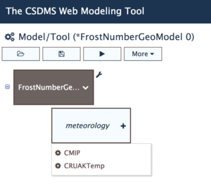
If you have done the previous labs, you now are familiar with the approach of the Air Frost number, it uses the mean annual air temperature of a location (MAAT), as well as the yearly temperature amplitude. In the Air Frost parametrization the mean monthly temperature of the warmest month and coldest month set that amplitude. In the model coupling here we have assumed the warmest month is July and the coldest month is January. The 'degree thawing days' are above 0 C, the 'degree freezing days' are below 0 C. To arrive at the cumulative freezing degree days and thawing degree days, the annual temperature curve is approximated by a cosine as defined by the warmest and coldest months, and one can integrate under the cosine curve (see also in Frost number presentation). The CMIP component is a 'data component' processed from the CRU-NCEP Climate Model Intercomparison Project - 5, also called CMIP 5. Data presented include the mean annual temperature for each gridcell, mean July temperature and mean January temperature over the period 1902 -2100. This dataset presents the mean of all the CMIP5 models, and the original atmosphere ocean models were run for the representative concentration pathway RCP 8.5. In RCP 8.5, greenhouse gas emissions continue to rise throughout the 21st century.

>> Link the Frost number GEO component with the CMIP component >> In the Frost number component parameters adapt the time to start in 1950, for 150 years. Set the model dimensions to xdim=40 and ydim=30. Make sure you request the frost-number-air output file.

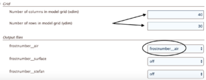
>> Then open up the settings for the CMIP5 data component. Make sure you start reading the data from 1950 onwards. Make sure you match the xdim and ydim with the Frost number grid dimensions. In addition, you will need to specify what region in large PanArctic dataset you do want to read. The CMIP5 data are on a half-degree latitude-longitude grid, so it consist of 720 by 360 grid cells. The upper left corner of the grid is at the international date line. For Alaska, set the column offset as 26, and the row offset as 32. Of course, the climate models keep track of 100's of physical variables; for our simple approximation we only need temperature. So this data component is subsampled to only provide monthly air temperature to other components. In the component here, the data is masked to only comprise the present-day permafrost region. The rest of the grid has 'no data' values.

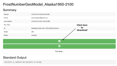
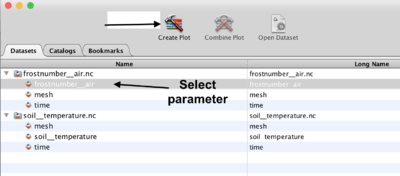
Download the zip file with your simulation output from the run status window. If you unzip the file you will find your output files, we will use the one called 'frostnumber__air.nc'. You can open this file with Panoply and plot the steady Frost number over 150 years by clicking on the 'create plot' icon

 What are typical mean annual temperatures over the North Slope of Alaska in the 1950's?
 Do you see much change in the mean annual temperatures at the end of the 21st century? 

 What does the Frost Number map look like for 1955, and for 2095? 
 What do these specific Frost numbers imply for the likelihood of permafrost occurrence?

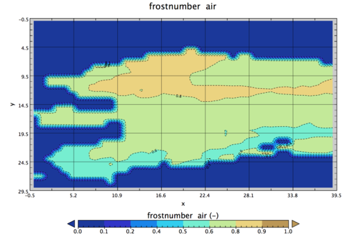
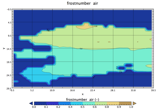
Permafrost scientist recently compiled an Arctic-wide inventory of the amount of carbon stored in the upper 3 m of soil in the permafrost regions, based on 100's of in-situ soil samples from all countries around the Arctic (Hugelius et al., 2016). The map below shows the distribution of carbon throughout soils across the Arctic region. It turns out permafrost soils are rich in organic carbon, and whereas these soils are currently still frozen, this carbon stock would possibly become available to decay with permafrost thaw in the future.

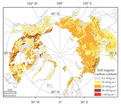
The total carbon storage is estimated to be 1035 +/- 150 Pg in the uppermost 3m of the permafrost zone, which means gross average carbon density is ~0.025 +/- 0.004 Pg per km3. If we are conservative, regions with Frost Number > 0.67, which we use here as a threshold for occurrence, declines about 6.68 million km2 by the end of the twenty-first century.

We assume that the disappearance of permafrost (as predicted by the Frost number) indeed means all 3m of soil is thawed. 
What would be a rough estimation of the amount of new carbon potentially exposed to the global atmosphere and carbon cycle?
How does that amount compare to the total amount of carbon in the atmosphere? (Hint, see Schuur et al., 2015).  

Discuss the factors that would make this first-order estimation problematic? 

References and More information

• Nelson, F.E., Outcalt, S.I., 1987. A computational method for prediction and prediction and regionalization of permafrost. Arct. Alp. Res. 19, 279–288.
  
• Schuur, E. A. G. et al. 2015, Climate change and the permafrost carbon feedback, Nature, 520(7546), 171–179, doi:10.1038/nature14338.
  
• Taylor, K. E., R. J. Stouffer, and G. A. Meehl. 2012, An overview of CMIP5 and the experiment design, Bull. Am. Meteorol. Soc., 93(4), 485–498, doi:10.1175/BAMS-D-11-00094.1.
• Wei, Y., Liu, S., Huntzinger, D. N., Michalak, A. M., Viovy, N., Post, W. M., Schwalm, C. R., Schaefer, K., Jacobson, A. R., Lu, C., Tian, H., Ricciuto, D. M., Cook, R. B., Mao, J., Shi, X., 2014. The North American Carbon Program Multi-scale Synthesis and Terrestrial Model Intercomparison Project – Part 2: Environmental driver data. Geosci. Model Dev., 7, 2875–2893. 10.5194/gmd-7-2875-2014

More on Model code and Running this model

Documentation for this model can be found Frost_Model metadata in CSDMS repository.
If you'd like to run this code or contribute to it, find it in our repository: Permafrost Modeling Toolbox Codes