Labs WMT ROMSLIte RiverPlume

Introduction to Regional Ocean Modeling - River Plume 2 base case and ROMS grids

This lab has been designed and developed by Courtney Harris and Julia Moriarty, Virginia Institute of Marine Sciences, Gloucester Point, VA
with assistance of Irina Overeem, CSDMS, University of Colorado, CO

Classroom organization
This lab is the first in a series of introduction to the Regional Ocean Modeling System (ROMS) for inexperienced users. ROMS is a three-dimensional hydrodynamic ocean model. It solves the conservation of mass and 3D momentum equations and includes transport equations for temperature and salinity. Here we present a basic configuration of ROMS in the framework of the Web Modeling Tool (WMT), it is designed for inexperienced modelers to look at a river plume affecting the coastal ocean and sediment transport. Basic theory is presented in these slides File:ROMS Lite Introduction.pptx.
This lab will likely take ~ 3hours to complete in the classroom.
If you have never used the Web Modeling Tool, learn how to use it here. The WMT allows you to set up simulations, but once you are ready to run them, you will need an account on the CSDMS supercomputer to submit your job. More information on getting an account can be found here HPCC Access. Note that getting permission for access takes a few days after your application.

Learning objectives

Skills

• familiarize with a basic configuration of the Regional Ocean Modeling System
• hands-on experience with visualizing NetCDF output with Matlab or Panoply.

Topical learning objectives

• learn about grids in oceanographic modeling
• integration of the conservation of momentum, continuity equation and conservation of tracers into a specific advection-diffusion scheme
• learn about a river freshwater plume evolving into a marine basin

Lab Notes

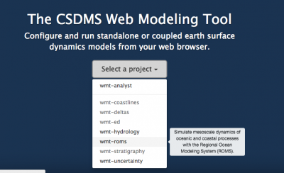
>> Open a new browser window and open the Web Modeling Tool here and select the ROMS project
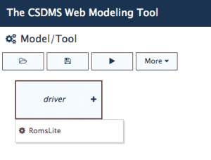
>> This WMT project is unique in that there is only a single driver, ROMS-Lite. It is a pre-compiled instance of the larger ROMS system specially configured for teaching use.

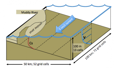
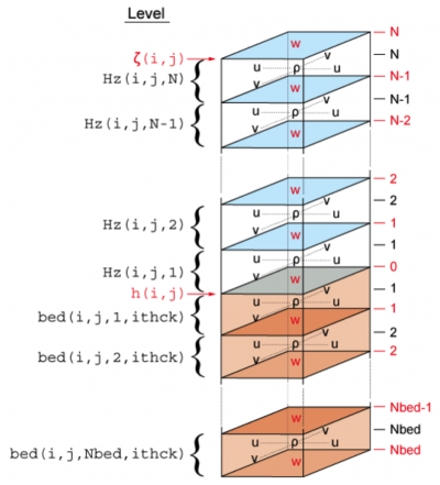
We set up a basic numerical experiment with inputs considered representative for a medium-sized river draining into the coastal ocean. The incoming river carries freshwater and suspended sediment into the salty ocean water. The river discharge is kept constant over the duration of the simulation at 1500 m3/sec. The model domain is 52 by 72 gridcells, gridcells are dx=500m and dy= 750m. This experiment ROMS has 20 vertical layers in the water column, and stores 10 layers in the ocean bed.

Scetch the planview grid set-up in ROMS for a single grid cell (hint this setup is known as an Arakawa-C grid). How/where do you evaluate salinity in one of these grid cells?

>> Run the base case configuration. It is on purpose set up to be short and fast (it takes only a few minutes to run). Download the zip file with your simulation output from the run status window

The ocean_riverplume2.nc file has bundled all important output. Typically the tracer quantities, like salinity and suspended sediment concentration, can be plotted as a 2D plot of eta-rho (x-axis) and xhi_rho (y-axis).

Plot a stack of planview maps of salinity, how far out offshore does the river plume still affect the ocean conditions? Until what depth is salinity noticeably affected?

This feature is a coast-hugging plume, or also called a 'surface trapped plume'. Why? Do you know of real-world  examples of coast-hugging plumes? 

>> Set up an additional WMT ROMS-Lite simulation for the same river and ocean conditions, but double the suspended sediment concentrations. Run this simulation and download the output.

Plot plan view maps of the final time slice for the mud001 concentration, do this both for our 'base case' as well as for the 'high concentration' simulation. How do the two results differ from each other? Does a river plume with a higher sediment concentration travel further out offshore? What do you think controls this distance?

References and More information

• The regional oceanic modeling system (ROMS): a split-explicit, free-surface, topography-following-coordinate oceanic model, A. F. Shchepetkin, J. C. McWilliams, Ocean Modelling 9 (2005) 347–404
• Much more information on ROMS community help pages
• Arakawa, A.; Lamb, V.R. (1977). "Computational design of the basic dynamical processes of the UCLA general circulation model". Methods of Computational Physics 17. New York: Academic Press. pp. 173–265.