Labs WMT Permafrost FrostNumberGEO
Introduction to Permafrost Processes - Lesson 3 Permafrost Maps using the Frost Number Model
This lab has been designed and developed by Irina Overeem and Mark Piper, CSDMS, University of Colorado, CO
with assistance of Kang Wang, Scott Stewart at CSDMS, University of Colorado, CO, and Elchin Jafarov, at Los Alamos National Labs, NM.
These labs are developed with support from NSF Grant 1503559, ‘Towards a Tiered Permafrost Modeling Cyberinfrastructure’
Classroom organization
This lab is the third in a series of introduction to permafrost process modeling. In this third lesson, we further use the Air Frost number model and learn to use this model to create spatially varying predictions of permafrost within the CSDMS Web Model tool (WMT). We implemented the Air Frost number model (as formulated in Nelson and Outcalt, 1987). This pseudo-2D implementation is named the Frost-number GEO model.
This series of labs is designed for inexperienced modelers to gain some experience with running a numerical model, changing model inputs, and analyzing model output. Specifically, this lab combines the simple model with a climate reanalysis dataset, modified from the CRU-NCEP climate data over the 20th century.
Basic information on the CRU_AK data component is presented in these slides. File:FrostNumberGEOModel Lecture3.pptx
This lab will likely take 1,5 -2 hrs to complete in the classroom. This time assumes you now have gained some familiarity with the WMT and have learned how to set parameters, save runs, download data and look at output. If this is not the case, either start with Lab 1 in this series, or do the WMT Tutorial
Learning objectives
Skills
- familiarize with a basic configuration of the Air Frost number Model for a gridded region.
- hands-on experience with visualizing NetCDF time series with Panoply.
- data to model comparisons and how to think about uncertainty in data and model output.
Topical learning objectives:
- what is a climate reanalysis product, what uncertainties does it have?
- what are regional differences in permafrost occurrence
- what are important parameters for assessing the state of permafrost in the future?
Lab Notes
>> The following questions can be answered from looking at the presented slides, to learn what climate/meteorological data is being used in this lab.
How many WMO meteorological stations do you think are available for Alaska? The state of Alaska comprises 1.7 million km^2.
The resolution of the dataset is for the purpose of this lab brought down to ~ 10km (to keep information exchange reasonable).
 How would the data sparseness affect model to observed data comparison?
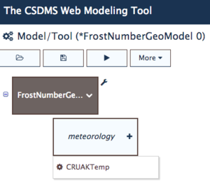
>> Set up a simulation that couples the Frostnumber-GEO model with the CRU_AKtemp reanalysis data. You will select the frost number GEO component as the driver, and see that it needs another component, called meteorology, to provide information. In our case the meteorological parameters are provided by the CRU-AKtemp data component. Once you have connected it to the Frost model, you can set each's components configuration by clicking on their respective 'set parameters'.
Take care to set the grid dimensions to be equal in both components, to cover most of the domain use 140 by 140 gridcells
 |
 |
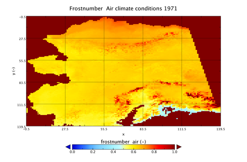
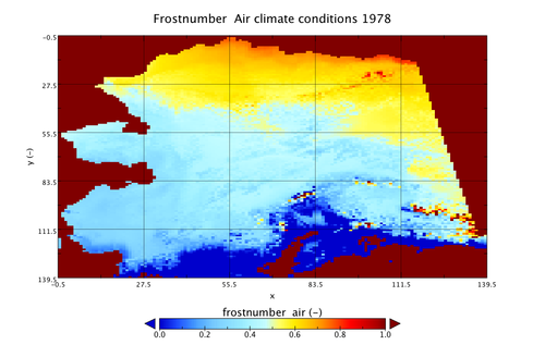
>> We will run the Frost number calculations for 1970-1980, sampling out of the CRU_AK reanalysis data. Set up the simulation for 10 years, starting in 1970 and with yearly output. Run the simulation, download the output. Open the file forstnumber__air.nc in Panoply. You will need to plot x versus y to get a map view of Alaska.


 Why are the maps for the Frost number for 1971 and 1978 so different?
 What is the likelihood for permafrost occurrence in the Alaska range? How do you explain this?
References and More information
- Nelson, F.E., Outcalt, S.I., 1987. A computational method for prediction and prediction and regionalization of permafrost. Arct. Alp. Res. 19, 279–288.
- Daly, C., et al., 2008. Physiographic sensitive mapping of climatological temperature and precipitation across the conterminous US. Int. J. Climatol. DOI: 10.1002/joc.1688
- Harris, I., Jones, P, Osborne, T, Lister, D., 2014. Updated high-resolution grids of monthly climaticobservations – the CRU TS3.10 Dataset. J. Climatol. 34: 623–642.
- Chadburn, S.E., Burke, E.J., Cox, P.M., Friedlingstein, P., Hugelius, G., Westerman, S., 2017. An observation-based constraint on permafrost loss as a function of global warming.Nature Climate Change, 10 APRIL 2017 | DOI: 10.1038/NCLIMATE3262
More on Model code and Running this model
Documentation for this model can be found Frost_Model metadata in CSDMS repository.
If you'd like to run this code or contribute to it, find it in our repository: Permafrost Modeling Toolbox Codes
