Labs WMT Hydrology StreamResponsetoRain
Hydrology Modeling - Stream Response to Rainfall Event
Classroom organization
If you have never used the Web Modeling Tool, learn how to use it here. The WMT allows you to set up simulations, but once you are ready to run them, you will need an account on the CSDMS supercomputer to submit your job.
More information on getting an account can be found here HPCC Access
This lab is one of the more advanced labs in a series of hydrology labs, it will likely take ~ 3hours to complete fully. These labs use TOPOFLOW components to simulate basic hydrological processes such as the energy budget, precipitation, snowmelt, evaporation, infiltration etc.
TOPOFLOW components are designed to be coupled and to model water runoff in a landscape, i.e. in a 'spatially-distributed' hydrological model. This lab couples the meteorology component and the channels kinematic wave component to model the runoff in response to a rainstorm.
In the model simulations we will generate 3 different rainfall events and see how the runoff in a small watershed is routed.
Learning objectives
- concepts of watershed and runoff
- relation between rain and runoff in absence of evaporation and infiltration
Key concepts
- Conservation of Mass
Lab Notes
>> Open a new browser window and open the Web Modeling Tool WMT with hydrology components
>> We will start out with an example called 'HydrologyLab_Channels_Treynor_ConstantRain'
This simulation couples the Channels Kinematic Wave Component and the Meteorology component in the WMT. You can browse through the Parameter List and learn how this simulation is set up. This is an basic run for a watershed in Iowa, called Treynor watershed. It is a small Agricultural Research Watershed in the Corn Belt in Iowa, and it consist of deep loess soils, and is mostly single-cropped. Treynor watershed has been a study watershed for many decades for rain, runoff and erosion observations. Rainfall - runoff observations here are very detailed and can thus potentially be used to benchmark hydrological models. The DEM for Treynor has been pre-loaded and is the default grid in the WMT-hydrology (it is called 'site').
The duration of this simulation is set at 3 hours (10,800 seconds). Note that the Channels Kinematic Wave component, which routes the water over the landscape needs small time steps (here set at every 6 seconds), whereas the Meteorology component, which provides the rainfall runs at a coarser time-resolution (every 60 seconds).
We will calculate the meteorological conditions with most of the parameters set by just single values. This first simulation rains on the landscape at a uniform rain rate of 54 mm/hr.
>> Save this configuration as a personal example. Then, you can run it by hitting the run button. This way you generate a job script that can be submitted to Beach-the CSDMS High Performance Computing System. Provide your HPCC account information (i.e. user name and password) to get the run started. The status page allows you to keep track of a simulation. From the status page you can eventually download your output files.
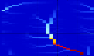
Water discharge is calculated by the channels kinematic wave component and is presented in the netcdf file called 'channel_water-_x-section__volume-flow-rate.nc'. We saved output every 10 minutes, so there si a total of 18 time slices in 3 hours. You can plot these output files in Panoply. The figure below shows an example of the water discharge distribution in this small watershed. It can easily be seen that the upstream hillslopes have less discharge, whereas the downstream river accumulates the discharge of several tributaries.
Plot a hydrograph, a timeseries of discharge, for an upstream gridcell and a gridcell at the watershed outlet. Explain the difference between the upstream and downstream cells. Is the hydrograph pattern to be expected for a uniform rain rate?
>> Open the second pre-loaded example, called 'HydrologyLab_Channels_Treynor_JuneRainStorm'. Browse the input settings and run this simulation.
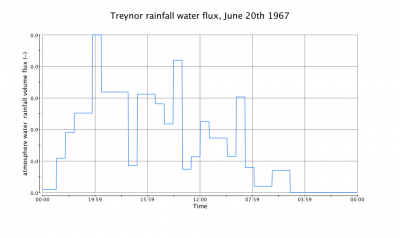
Whereas we applied a constant rain rate before, we now upload a time-series with variation of rain rate within the 3 hours. TOPOFLOW components typically can use scalars, time-series or even grids over time for many input parameters. Now we will run a real-world observed rainstorm, which has been measured in June 1967. Rain fall input as used in the Meteorology component is saved in the parameter: 'atmosphere water__rainfall_volume_flux.nc'.
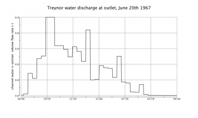
Plot the hydrographs for the same two grid cells, one more upstream, one more downstream you had looked at before. What are the differences?
If you compare the rainfall input directly to the discharge, do you see any dampening? Why is there such a direct response to the rainfall?
>> You can use the second pre-loaded example as a base-case and upload your own time series of rain fall data. Set up a text file (in Text Wrangler or on a UNIIX system) for 180 minutes. If you want to run precisely the same amount ofwater as the previous runs but just over a single hour, how high would your rain rate be?
You can either just plot results, or use some more advanced analysis of netCDF files to look at the total incoming flux and the total outgoing flux.
Does the rainfall-runoff predictions in these simulations conserve mass? If not, why not?


