Labs WMT CEM

Coastal Evolution

If you have never used the Web Modeling Tool, learn how to use it here. The WMT allows you to set up simulations, but once you are ready to run them, you will need an account on the CSDMS supercomputer to submit your job. More information on getting an account can be found here Beach HPCC Access
To learn more about the models in this lab, specifically the Coastal Evolution Model, CEM, you can download this presentation.

These experiments couple the terrestrial and coastal domains. we will be looking at a river supplying sediment to a coastal zone, along which wave-driven longshore transport occurs. We will learn about the effect of incoming wave fields, the effect of sediment supply to the coast, and whether this supply happens through a single delta channel or multiple delta channels.

>> Open a new browser window and open the Web Modeling Tool CSDMS WMT

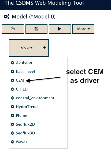
>> For this specific exercise we will be running the coupled CEM model. This means that you only choose CEM as the driver from the Component List.

.

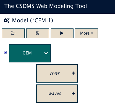
>> CEM will now be active in the WMT.
>> CEM needs to be connected to other components to set up a coupled simulation.

Once you have added the components you can set the parameters for each by going through the different tabs in the parameter list. Once your input is set up, you save the information. Then, you can run it by hitting the arrow run button. This way you generate a job script that can be submitted to Beach-the CSDMS High Performance Computing System. Provide your Beach account information (i.e. user name and password) to get the run started. The status page allows you to keep track of a simulation. From the status page you can eventually download your output files.

'Exercise 1: Generate a wave-dominated delta

>> Run a “base-case” simulation for 6000 time-steps .
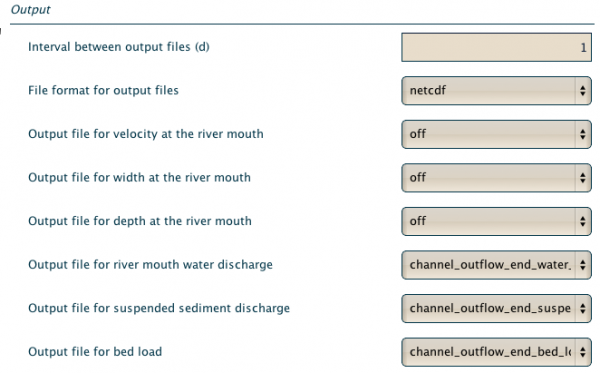
>> Use a constant high river bedload input of 300 kg/s. Use a modest wave height (1 m, 8 seconds). Run your scenario for a single channel with no avulsion. >> Scroll down to find the output settings. Specify a number of output files to generate after the simulation: these are netCDF files of water discharge, suspended sediment, and bedload. Make sure the output interval is set to 250 (every 250 timesteps).

>> Now run the simulation!
>> Download the output files. You can use VisIT to visualize your results.

Question 1a

Do you think the values for bedload flux and wave height are realistic? If not, why not? Can you give an example of a river or delta system that would be experiencing this influx of bedload and a comparable wave regime?

Question 1b

Plot up your results in VisIT. Is the evolved delta planview map reminiscent of a wave-dominated delta?

Question 1c

Make a movie of the evolution of the delta systemevolving over time. Export the movie as a mpeg file.

Exercise 2: Explore the influence of wave regime on delta formation

Now we will look at changing the wave conditions. Systematically vary the wave regime: the asymmetry of the incoming wave angle (A) and the highness factor for the incoming waves (U). A ranges from 0-1. A >0.5 indicates that the majority of wave energy is approaching from the left where a designation of 1.0 indicates all wave energy approaches from the left. A = 0.5 indicates wave energy approach is evenly distributed between the left and right. A < 0.5 indicates the majority of wave energy is approaching from the right where a designation of 0.0 indicates all wave energy approaches from the right. U controls the directional spread of the approaching waves, here split into whether waves approach from angles great than or less than the one which maximized alongshore sediment transport (~ 45 deg). High-angle waves approach with angles greater than 45 degrees and low-angle waves approach more directly onshore. U< 0.5 indicates wave energy predominately approaching from a low angle, U> 0.5 indicates a predominance of high-angle waves. For scenarios involving delta evolution, values less than 0.5 tend to be more reasonable.

>> design a matrix of 9 experiments with varying A and U values.

Question 2a
Plot up your last time step for each of your experiments and describe the different delta shapes.

Exercise 3: Explore the influence of channel avulsions on delta formation

Pick a base-case from your previous experiments (be sure to document your settings). Run a simulation where you assign a much higher likelihood of channel switching by changing the standard deviation of avulsion angles.

Question 3a Can you describe a real-world delta system that would have a single channel and a high switching rate? Why does this happen? If yes, add a GoogleEarth image to your notes. Plot up your final time step and describe the delta geometry.

Question 3b

How does delta progradation change with multiple distributary channels? Run a simulation with 3 distributary channels and compare progradation rates to your ‘one-channel’ experiment. Make a movie of the evolution of the delta with multiple distributaries evolving with VisIt. Export the movie as an mpeg.

Exercise 3: How do humans affect river sediment loads?

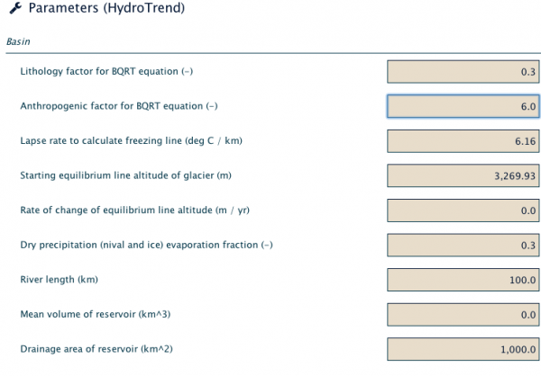
Here we will look at the effect of human in a river basin. Humans can accelearate erosion processes, or reduce the sediment loads traveling through a river system. Both concepts can be simulated, first run 3 simulations systematically increasing the anthropogenic factor (0.5-8.0 is the range).

Question 3a
Describe in your own words the meaning of the human-induced erosion factor, (Eh) (Syvitski & Milliman, 2007). 
This factor is parametrized as the  “Antropogenic” factor in HydroTrend. See references for the paper.

>> Model a scenario of a drinking water supply reservoir to be planned in the coastal area of the basin. The reservoir would have 800 km ²of contributing drainage area and be 3 km long, 200m wide and 100m deep. Set up a simulation with these parameters.

Question 3b
How would such a reservoir affect the sediment load at the coast (i.e. downstream of the reservoir)?