Labs WMT CEM: Difference between revisions
(working on the updated CEM lab) |
|||
| (30 intermediate revisions by 2 users not shown) | |||
| Line 1: | Line 1: | ||
==Coastal Evolution== | ==Coastal Evolution== | ||
The Coastline Evolution Model (CEM) addresses predominately sandy, wave-dominated coastlines on time-scales ranging from years to millenia and on spatial scales ranging from kilometers to hundreds of kilometers. Shoreline evolution results from gradients in wave-driven alongshore sediment transport. The model has been used to represent varying geology underlying a sandy coastline and shoreface in a simplified manner and enables the simulation of coastline evolution when sediment supply from an eroding shoreface may be constrained. CEM also supports the simulation of human manipulations to coastline evolution through beach nourishment or hard structures. To learn more about the models in this lab, specifically the Coastal Evolution Model, CEM, you can download this [[:File:CoupledAvulsionCEMWMTversion.pptx|presentation]]. | |||
To learn more about the models in this lab, specifically the Coastal Evolution Model, CEM, you can download this [[:File:CoupledAvulsionCEMWMTversion.pptx|presentation]]. | |||
This lab includes experiments to couple the terrestrial and coastal domains. We will be looking at a river supplying sediment to a coastal zone, along which wave-driven longshore transport occurs. We will learn about the effect of incoming wave fields, the effect of sediment supply to the coast, and whether this supply happens through a single delta channel or multiple delta channels. Many deltas are classified as wave-dominated deltas, the Arno Delta in Italy is one example.<br> | |||
<br> | |||
[[file:ArnoRiverDelta.png| Arno delta]] | |||
<br> | |||
[ | This lab will run CEM simulation with Python Modeling Tool (Pymt). If you have never used the Pymt, learn how to use it [https://pymt.readthedocs.io/en/latest/install.html here]. The Pymt allows you to set up simulations and run notebooks. | ||
If you are a faculty at an academic institution, it is possible to work with us to get temporary teaching accounts. Work directly with us by emailing: csdms@colorado.edu | |||
'''Learning objectives'''<br> | |||
Skills: | |||
*use Pymt to run CEM Model | |||
*familiarize with a basic configuration of the CEM Model | |||
*make changes to key input parameters | |||
*hands-on experience with visualizing output in Python | |||
Topical learning objectives: | |||
*generate a wave-dominated delta | |||
*explore the influence of wave conditions (e.g., wave height, wave angle) on delta formation | |||
*explore the influence of river input on delta formation | |||
'''Lab Notes''' | |||
You can launch binder to directly run the Jupyter Notebook for this lab through a web browser. | |||
>> Open a new browser window and open the Pymt read the docs page [https://pymt.readthedocs.io/en/latest/examples.html here] | |||
[[File:launch_binder_cem.png|400px]] | |||
>> You will see that there are several example models. In this lab we will select the Coastline Evolution Model. <br> | |||
>> Click on the 'Launch Binder' box and it will allow you to see this lab as a Jupyter Notebook.<br> | |||
<br><br> | >> You can execute the Jupyter notebook code cells using shift -enter. | ||
'''References'''<br> | |||
* Ashton, A, A.B. Murray, and O. Arnoult. 2001. Formation of coastline features by large-scale instabilities induced by high-angle waves. Nature 414: 296-300., 10.1038/35104541 | |||
* Ashton, A.D. and Murray, A.B., 2006. High-angle wave instability and emergent shoreline shapes: 2. Wave climate analysis and comparisons to nature. Journal of Geophysical Research 111. F04012., 10.1029/2005JF000423 | |||
<br> | |||
'''More on Model description and code''' | |||
* [https://github.com/csdms/cem-old/tree/mcflugen/add-function-pointers CEM source code]: Look at the files that have *deltas* in their name. | |||
* [http://csdms.colorado.edu/wiki/Model_help:CEM CEM description on CSDMS]: Detailed information on the CEM model. | |||
Latest revision as of 18:44, 19 March 2020
Coastal Evolution
The Coastline Evolution Model (CEM) addresses predominately sandy, wave-dominated coastlines on time-scales ranging from years to millenia and on spatial scales ranging from kilometers to hundreds of kilometers. Shoreline evolution results from gradients in wave-driven alongshore sediment transport. The model has been used to represent varying geology underlying a sandy coastline and shoreface in a simplified manner and enables the simulation of coastline evolution when sediment supply from an eroding shoreface may be constrained. CEM also supports the simulation of human manipulations to coastline evolution through beach nourishment or hard structures. To learn more about the models in this lab, specifically the Coastal Evolution Model, CEM, you can download this presentation.
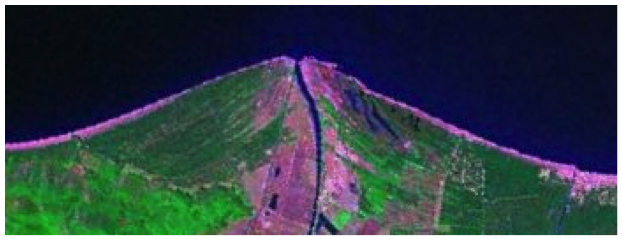
This lab includes experiments to couple the terrestrial and coastal domains. We will be looking at a river supplying sediment to a coastal zone, along which wave-driven longshore transport occurs. We will learn about the effect of incoming wave fields, the effect of sediment supply to the coast, and whether this supply happens through a single delta channel or multiple delta channels. Many deltas are classified as wave-dominated deltas, the Arno Delta in Italy is one example.

This lab will run CEM simulation with Python Modeling Tool (Pymt). If you have never used the Pymt, learn how to use it here. The Pymt allows you to set up simulations and run notebooks.
If you are a faculty at an academic institution, it is possible to work with us to get temporary teaching accounts. Work directly with us by emailing: csdms@colorado.edu
Learning objectives
Skills:
- use Pymt to run CEM Model
- familiarize with a basic configuration of the CEM Model
- make changes to key input parameters
- hands-on experience with visualizing output in Python
Topical learning objectives:
- generate a wave-dominated delta
- explore the influence of wave conditions (e.g., wave height, wave angle) on delta formation
- explore the influence of river input on delta formation
Lab Notes
You can launch binder to directly run the Jupyter Notebook for this lab through a web browser.
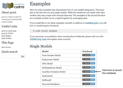
>> Open a new browser window and open the Pymt read the docs page here
>> You will see that there are several example models. In this lab we will select the Coastline Evolution Model.
>> Click on the 'Launch Binder' box and it will allow you to see this lab as a Jupyter Notebook.
>> You can execute the Jupyter notebook code cells using shift -enter.
References
- Ashton, A, A.B. Murray, and O. Arnoult. 2001. Formation of coastline features by large-scale instabilities induced by high-angle waves. Nature 414: 296-300., 10.1038/35104541
- Ashton, A.D. and Murray, A.B., 2006. High-angle wave instability and emergent shoreline shapes: 2. Wave climate analysis and comparisons to nature. Journal of Geophysical Research 111. F04012., 10.1029/2005JF000423
More on Model description and code
- CEM source code: Look at the files that have *deltas* in their name.
- CEM description on CSDMS: Detailed information on the CEM model.

