Labs ERODE
Landscape Evolution Modeling with ERODE
This lab introduces you to the landscape evolution model ERODE. ERODE is a raster-based landscape evolution model; it evolves a landscape with a combination of hillslope erosion and transport and river channel erosion and transport.
The Help Page of ERODE can be found here
STEP1 Load the ERODE project
Once you are in the CSDMS Modeling Tool:
>> Under the File Menu, choose ‘Open Project’.
>> Go to the Terrestrial Group. Open Project: ERODE
>> Drag the ERODEGlobal component in the driver palette
>> Specify a unique working directory for each experiment, for example: /CMT_Output/ERODEexp1 (…etc for the next experiment).
Learn about Flow Routing with ERODE
An important part of ERODE is the way it treats routing of water (and sediment) through the landscape. To give you a bit of a feel of the methodology, we will look at the ‘D8 method’ for determining the drainage directions in a raster grid.
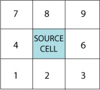
Assume you have a 3 by 3 grid. So if one has a source cell of interest in the middle, we assume that water and sediment drains in the direction of the steepest slope. This concept is also called ‘steepest descent’. The grid cell in the middle then has 8 neighboring cells, and depending on their elevations (z), and the distance between the cells, d, you can calculate the slope, S.
[math]\displaystyle{ S = \Delta z / d }[/math] (1)
These surrounding cells are coded as shown in the figure here:

Question
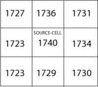
In the hypothetical elevation grid below, the source cell and its 8 neighbors have defined elevation values.
Where does the water drain to? Select the correct cell and list its D8- grid value.
Question
Can you think of a theoretical situation when a D8 flow direction algorithm would not work?
What would such a situation look like in a real DEM?
STEP2 Run and analyze an ERODE simulation
Landscapes evolve over long periods of time, and to optimize how long a simulation takes one would like to have large timesteps. However, if the elevation differences created by erosion and sedimentation become too large, the numerical scheme can cause instabilities. One approach is to use adaptive time-stepping methods, where time-steps are large when relatively little happens, and time-steps are short when the landscape evolves more rapidly. ERODE uses such an adaptive time-stepping scheme.
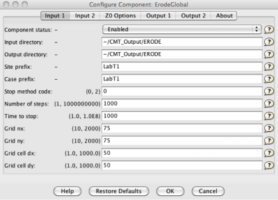
>> Start two short simulations of ERODE. Use stop-method code 0, and use 1000 time-steps as your simulation duration. Use for the first simulation a grid of 75 by 75 cells and for the second simulation a grid of 50 by 50 cells. Ask for output grids every 100 years (use the z-grid for elevations and the A-grid for contributing Area).

Question
For a grid of 75 rows by 75 columns, each of 50m by 50m, how much time can be simulated in 1000 time-steps (under the default conditions set for ERODE in CMT)?
How much time for the smaller grid? (Hint: this should be reported in the joblist when you click on the relevant job).
In the ERODE Input tab 2 you will see a field to choose the CLF-criterion. This is a form of a stability condition, called the ‘Courant-Friedrichs-Lewy Condition’. This condition in numerical equation solving states that, given a space discretization, a time step bigger than some computable quantity should not be taken.
Question
Find the definition of the CFL condition and predict what would happen to your simulated time if you’d use a higher CLF. (Of course, you can do a simulation and see whether that prediction pans out).
Dominance of hillslope processes versus channel processes
Major process controls in ERODE come from the formulation of the discharge, Q, and sediment fluxes, Qs, over the landscape. Discharge is a function of the rainrate R [L/T], and contributing area A [T2]:
[math]\displaystyle{ Q = R \cdot A^p }[/math] (2)
Sediment flux is controlled by the slope, S, [-], discharge Q, and the erodibility K:
[math]\displaystyle{ Q_{s} = K \cdot Q^m \cdot S^n }[/math] (3)
>> Start two longer simulations of ERODE. Use stop-method code 0, and use 20,000 time-steps as your simulation duration, much longer than your previous runs. Ask for output every 500 years. Use a grid of 60 by 60 cells. Vary the area-exponent and the slope exponent independently. (In ‘inputtab 2’ use a base-level lowering of 0.05mm/yr, a rainrate of 2m/yr).
>> Visualize the output grid stacks in Visit. There are two useful NetCDF files generated, an elevation file, called:*_2D-z.nc’ and an contributing area file, called *_2D-A.nc
Question
What is the impact of a larger area exponent, m, compared to a larger slope exponent, n?
If there are hardly any differences, try making the runs longer or to vary other parameter you think influence this.
Please list your simulation setup parameters and plot the comparison figures of both elevation and contributing area   of your two final runs.

