Labs Basic CMT

Using the CSDMS Modeling Tool: Runoff Modeling with TOPOFLOW

STEP1 Load the TOPOFLOW project

Go to the CMT Workspace and Open TOPOFLOW Project Now you are in the CSDMS Modeling Tool. It will automatically start up in the CMT Help, for the exercises we will use the ‘CMT Workspace’.

• Under the File Menu, choose ‘Open project’.
• Go to the Terrestrial Group. Open Project: TOPOFLOW + GC2D.

You are ready to import examples, adapt and run simulations We will use the hydrological toolkit called ‘TOPOFLOW’ as an example to explore how CMT works, and what component modeling is all about.

STEP2 Run and visualize a TOPOFLOW simulation

Under the File menu, choose ‘Open Example Configuration’. Here examples of previously wired model simulations are stored. These files are called *.bld files.

>> Open the directory for TOPOFLOW.
>> Find the subdirectory 00_Oct_27_2011
>> Click on the ‘bld’ file named: Treynor_June_20_67_Storm_Oct_27_11.bld

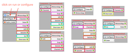
The Bld file brings up the pre-wired configuration as shown below. The TOPOFLOW component is the driver of this simulation. It needs to get values for all ‘Uses Ports’ on the righthand side of the component, i.e. meteorology, channels, snow…etcetera. The components in the Arena provide this information to the main driver.

This pre-wired TOPOFLOW simulation models a rainfall events in a small Agricultural Research Service watershed located near Treynor, Iowa. Data from Treynor watershed are ‘classic’ datasets that have become benchmark test cases for hydrological runoff and watershed models. The watershed was ~0.43 km2. Basin geometry parameters we will not be able to change in this hands-on, but you can normally load a relevant DEM. All parameters that are shown by default in the CMT for this TOPOFLOW Configurations are based on the benchmark data for a measured rainstorm on June 20th, 1967.

>> Run this simulation.
>> To get information on your run, go from the workspace to the Job Info space. There your jobs on Beach are listed with their ID’s and you can manage and query them.
>> Highlight your topoflow job.
>> Basic information on this job will be reported in the console.

Question 1 What was the duration of this model simulation?
Why would hydrological models or runoff models not have a fixed time step?

Question 2 What was the maximum precipitation rate for this rainstorm?
What was the maximum discharge at the outlet for this rainstorm?

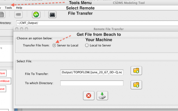
>> To get output from your run, transfer files from Beach to your local machine.
>> Under the CMT tools menu, choose remote file transfer, port files from your Beach account to your local machine.

>> After running your simulations, you now have the generated output files. The CMT tool generates the original output files as defined by the model developer. In addition, CMT generates NetCDF files as default format; these can be time-series or grid stacks. You can visualize NetCDF files a.o. with VisIT or with Matlab.

More information on VisIT and notes on installation: CMT visualization

>> Launch VisIT.
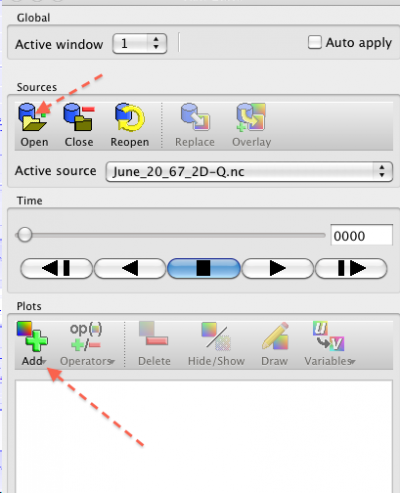
>> Under VisIT, choose ‘Open File’ and open ‘June_20_67_0D_Q.nc’.
>> This file will then show up as the Active Source.
>> You can use the Add button to add these variables to your plotting datasets.
>> Once you have added Q, you can use the ‘Draw button’ to plot a curve.

Question 3
What does the hydrograph for the June 20th, 1967 look like? What does the hydrograph look like in the upper part of the watershed? Plot both curves and export your figure. Does the maximum discharge match the reported maximum?

>> Under VisIT, choose ‘Open File’ and open ‘June_20_67_2D_Q.nc’

Question 4
Plot up this gridded variable. Use the play button to play it through the simulation time. What does the plot show?

Question 5
Why is it useful to simulate single rainstorm events?