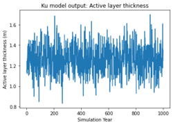
The Kudryavtsev et al. (1974), or Ku model, presents an approximate solution of the Stefan problem. The model provides a steady-state solution under the assumption of sinusoidal air temperature forcing. It considers snow, vegetation, and soil layers as thermal damping to variation of air temperature. The layer of soil is considered to be a homogeneous column with different thermal properties in the frozen and thawed states. The main outputs are annual maximum frozen/thaw depth and mean annual temperature at the top of permafrost (or at the base of the active layer). It can be applied over a wide variety of climatic conditions.
Classroom organization In this lab, it includes two Jupyter Notebooks. In the first notebook, we will explore the Ku model to simulate the active layer thickness and soil temperature. In the second notebook, we will use the active layer depth results from Ku model to drive a depth-dependent hillslope diffusion model over the Eight Mile Lake study site. The second notebook gives one very simplistic example for how Ku can be used alongside landscape geomorphology models.
If you are a faculty at an academic institution, it is possible to work with us to get temporary teaching accounts. Work directly with us by emailing: csdms@colorado.edu
Learning objectives Skills
Learn how to use "permamodel" Python module to run Ku model
Learn to load, rescale, and visualize DEM data in Python.
Learn how to use Ku model output and Landlab component to run depth-dependent diffusion model
Key concepts
What are important parameters for calculating active layer thickness
Lab notes You can follow the steps below to test and run the Jupyter Notebooks on the CSDMS JupyterHub server for this lab.
1. Create a free account on the CSDMS JupyterHub at https://csdms.rc.colorado.edu/hub/signup, providing a username and password -- they can be whatever you like