Island
Welcome to the Earthscape Simulator
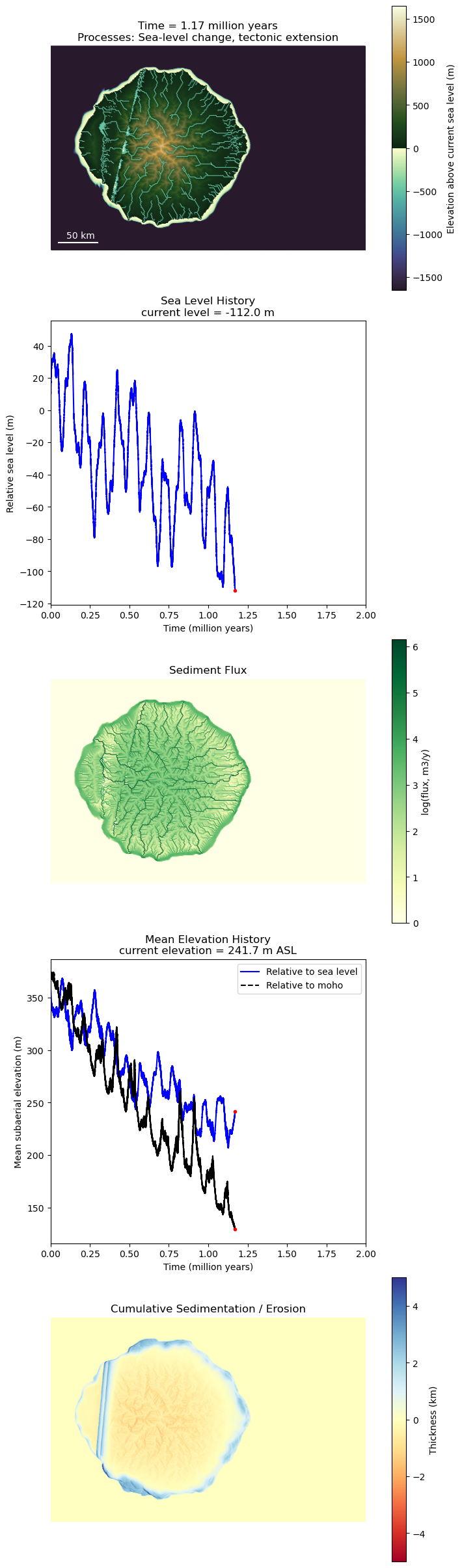
Earthscape Simulator, also known as "Brain Island", is a perpetually running computer model that simulates geological processes on an imaginary island. The simulation is meant to serve two purposes. First, it provides a way to visualize geologic change through processes such as tectonic uplift and subsidence, isostatic adjustment, sea-level variations, and erosion and sedimentation, both on land and in the adjacent ocean. Second, the model is meant to inspire conversation among the research community about how these "source-to-sink" processes can be represented mathematically and computationally, what processes might be missing or incompletely represented, and how we might improve on the model.
Scroll down to view the latest configuration of the island, and to read more about what goes into the simulation model.
What's in the model?
Earthscape Simulator is a Python-language computer program that uses a Landlab grid and Landlab components to model the ongoing geologic evolution of a hypothetical "chunk" of continental crust (or perhaps over-thickened oceanic crust?) embedded in ocean lithosphere. The starting condition consists of a roughly circular island, with a more or less cone-shaped topography, and some randomly generated bumps and depressions. The source code for the simulator and the initial-topography generation can be found on GitHub at https://github.com/gregtucker/earthscape_simulator.
Here are some of the processes and other elements in the currently running version model (as of February 2024):
Representing the landscape and seascape: The simulation uses a Landlab HexModelGrid, with hexagonal grid cells that are spaced 1 km apart.
Sea-level change: The current run uses a sea-level variation composed of a sum of sine curves in four of the (approximately) Milankovitch frequencies: 19, 22, 41, 100, and 405 thousand years; the amplitudes were chosen more or less arbitrarily to give maximum sea-level variation on the order of 120 meters. (Othe runs have used a sea-level history reconstructed for the past 10 million years. The history combines a high-resolution reconstruction for the last ~2 million years with a lower-resolution reconstruction for the remaining time.) The sea-level curve is interpolated onto the model's time steps, which are currently 50 years.
Epeirogenic uplift: The current run has a slow (0.00005 m/yr), steady, uniform rate of relative sea-level change to represent epeirogenic (i.e., regional) uplift, such as might occur due to temperature variation in the mantle. This is implemented by adding a long-term falling trend to relative sea level.
Rift tectonics: The island is subject to rifting, which is represented by a listric ("spoon-shaped", or in this case, exponential-function-shaped) detachment fault. The fault's precise location and strike angle are generated at random. Every so often (a time period also chosen at random), the fault will jump to the east by a certain (also random) amount. Hence, while rifting is active, a series of faults will develop. The fault plane, which dips eastward, has a 60-degree dip near the surface, but it flattens out with depth until it becomes a 10 km deep horizontal detachment. All material above this detachment surface - that is, everything in the hangingwall of the fault - moves eastward at a specified rate (the rate in the current run is 2.5 mm/year). Fault geometry and motion are computed by a Landlab component called ListricKinematicExtender, which in turn uses the AdvectionSolverTVD component to calculate the lateral advection of the hangingwall.
Flexural isostasy: Changes in the distribution of weight, due to a combination of rifting, erosion, and sedimentation, cause an isostatic response. This is calculated by treating the lithosphere as an elastic sheet overlying an inviscid fluid upper mantle. The calculation is handled by the Landlab Flexure component. Because Flexure requires a rectilinear grid, it is solved on a separate RasterModelGrid of the same domain size and average grid spacing as the hex grid used for the other processes.
Igneous intrusions: The model can generate random igeneous intrusions: underground blobs of magma that inflate the terrain above them. I'm indebted to Daniel O'Hara for suggesting this idea and sharing a movie of an "igneous intrusion landscape" simulation that he wrote. Here, the intrusions are conic parabolas of randomly determined diameter, depth, lifespan, and final thickness. They are implemented by an IgneousIntruder (which isn't quite a component yet, so it's included in the earthscape simulator codebase for now).
Flow of water across land: The routing of water across the land surface is calculated uses a flow-accumulation algorithm. Each grid cell above sea level is assigned a flow direction toward one of its six neighbors. The algorithm calculates and stores the downstream accumulation of drainage area, and multiplies this by a specified water runoff rate to compute an "effective" value of water discharge in each grid cell. These calculations are performed using the Landlab FlowAccumulator component. To handle the routing of water through closed depressions - in other words, lakes - the model uses a Landlab-native implementation of an algorithm developed by Richard Barnes; the component is called LakeMapperBarnes.
Erosion and sedimentation by rivers: The current version of the model calculates fluvial erosion, transport, and deposition using the "xi-q" formulation of Davy and Lague (2009), in which material is constantly exchanged between the water column and the river bed. Erosion occurs where the entrainment rate outpaces the sediment settling rate, and vice versa. This is implemented by the Landlab ErosionDeposition component.
The coastline - a moving boundary: The coastline represents a dynamically moving boundary, across which processes change. In order to "trick" the model into recognizing this moving boundary, all grid nodes below sea level are flagged as boundary nodes for purposes of calculating fluvial processes. Fluvial transport stops when the boundary is crossed. From a practical perspective, this is handled by collecting all the sediment passed to boundary nodes by river transport in adjacent land nodes, and depositing it locally, with a little bit of spreading out to reduce the "spikes" that tend to form where a large flow of sediment is dropped at a single point. (The speckled pattern in coastal areas arises from this fluvial deposition, and the speckling indicates that the current solution is far from ideal. It's a work in progress.)
Marine sediment transport: Transport of sediment below sea level is assumed to be driven by wave action, which entrains sediment into the water column, and gravity, which pulls it downslope. These processes are represented using a nonlinear diffusion equation, in which the quantity "diffused" is elevation (representing sediment volume at a given location). To represent the influence of waves, the diffusion coefficient is constant above a specified wave-base depth, and declines exponentially with depth where the depth is below the wave base. This process is implemented by the Landlab SimpleSubmarineDiffuser component.
Model speed: Can't it run any faster? Yes! Although normally we want our numerical codes to run as fast as possible, the Earthscape Simulator is a case where we want to slow it down a bit and enjoy the ride. Consequently, the maximum run speed is limited to a user-specified value (currently 5 model years per second).
What's missing?
Plenty! This is just a prototype. What about variable lithology? (Or even just rock versus sediment?) Orographic precipitation? Sedimentary facies and stratigraphy (the model makes stratigraphy but doesn't keep track of facies types or depositional ages)? Varying grain size? Landsliding? Bedrock plucking and abrasion? Downstream sediment abrasion?
Comments and questions are welcome!
If you have ideas on ways to improve on the model, or to improve on its visual representation, please share them! A good way to do this is to post an Issue on the model's GitHub repository site.
-Greg Tucker, University of Colorado Boulder, February 2024
