Coupling Rivers and Deltas with the CSDMS Modeling Tool

 

CEM - Steps to create a model is available here

1. Introduction

This manual illustrates how to couple two components bridging the terrestrial and marine domains. As a first example, we show here how to couple HydroTrend to the Coastal Evolution Model (CEM); thus coupling a river model with a delta model.

HydroTrend is a climate-driven river discharge and sediment load model. HydroTrend is 1 D and predicts water and sediment load at the river apex, before entering a delta or a marine basin.  It predicts both suspended load flux, for a number of grainsizes, and bedload flux.

HydroTrend has been designed and tested for rivers longer than 100km, and basins smaller than 75,000 km². HydroTrend generates time series of water and sediment flux, from 1000’s of years or just for a single year. The model can simulate at a daily resolution, but can also be set to give monthly or yearly output.

The Coastal Evolution Model simulates the evolution of predominately sandy, wave-dominated coastlines on time-scales ranging from years to millennia and on spatial scales ranging from kilometers to hundreds of kilometers.

Shoreline evolution results from gradients in wave-driven alongshore sediment transport. At its most basic level, the model follows the standard 'one-line' modeling approach, where the cross-shore dimension is collapsed into a single data point. However, the model allows the plan-view shoreline to take on arbitrary local orientations, and even fold back upon itself, as complex shapes such as capes and spits form under some wave climates.

 

2. Which Project?

-       You go to the Group ‘Terrestrial’ or the Group ‘Coastal’

-        Select the HydroTrend + CEM project

-Once you have entered this project, you will find amongst others the HydroTrend and CEM components in the component palette.

 

3. Coupling the HydroTrend and CEM Models

Drag the DeltaTrend-component into the CMT Arena. This is the model, that will orchester the simulation, and connects the terrestrial and coastal domains. When prompted you will identify this component as being the ‘driver’.

Drag the CEM-component into the CMT Arena. When prompted, specify that this is a component rather than a driver. The CSDMS Modeling Tool automatically recognizes that DeltaTrend uses a “CoastalModel” component, and this is provided by the “CoastalModel-provides port” of the CEM component. The connection happens and the ports when connected are highlighted in the same color. They may be shown wired if you work in the wired mode.

 

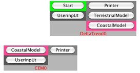
Fig 1. Coupling of the DeltaTrend ‘CoastalModel-uses-port’ and the CEM ‘CoastalModel–provides-port’.

Drag the HydroTrend-component into the CMT arena. This is the river feeding the coast or delta with incoming sediment. Again, when prompted, specify that this is a component rather than a driver.

It can be seen that all components need a printer connected to them in addition. So the last step is to drag in a printer component from the palette. Now the model is set-up and ready to go with its default input parameters(Fig 2).

This is how your example model would be set up if you use the ?????.bld file provided with this coupling as an example.

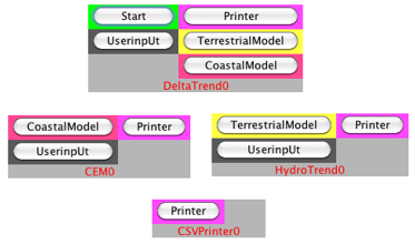
Fig 2. The final wiring diagram for a coupled HydroTrend-CEM simulation.

 

3. Specifying Simulation Parameters

Each component has a ‘Configure’ or ‘UserInput’ port where a user can specify simulation parameters. Depending on how far developed the integration of the component into the CMT has been established, there are more or fewer parameters that can be user-specified. Some of the CSDMS components are driven by their original input files, others have fewer input parameters and those are user-specified under the configure menus.

 

3.1 DeltaTrend Simulation Parameters and Input Files

As an example of a component that has relatively few input parameters; DeltaTrend has few input parameters and thse can be set directly by the user. If you open the ‘Configure’ or ‘UserInput’ port, you can set 1) the working directory, 2) the name under which you want this run to be labeled, this is called the simulation prefix, 3) the time span of your intended simulation (Fig. 3). You can see that this is set to be 10,000 days with output files being printed every 1000 days.

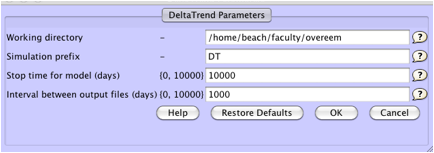
Fig 3. ‘Configure’ or ‘UserInput’ port of DeltaTrend component where a user can specify simulation parameters.

 

3.2 HydroTrend Simulation Parameters and Input Files

HydroTrend uses river drainage basin characteristics including relief, area and their distribution. This information is read from a hypsometric curve, i.e. a cumulative elevation–area distribution.  This information is presented in a plain ASCII file called: HYDRO.HYPS

In addition Hydrotrend needs a host of simulation settings on river basin climate characteristics, including temperature distributions and trends, and precipitation distributions and trends. This file is called HYDRO.IN

As you can see in the configure menu of HydroTrend, example input files are provided on the CSDMS HPCC system. They are located under the following directories:

beach:/data/sims/hydrotrend/Example1>

These files are based on runs for the Po river system, Italy.

beach:/data/sims/hydrotrend/Example2>

These files are based on runs for the Waiapoa river system, New Zealand.

 

3.3 CEM Simulation Parameters

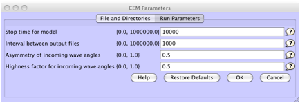
Fig 4. ‘Configure’ or ‘UserInput’ port of DeltaTrend component where a user can specify simulation parameters.

 

Figure 4 displays the configure menu of CEM, it is tabbed at the top, so you can go to multiple tabs to set parameters. The duration of the run and the stop time are here set to be similar to the DeltaTrend component. The wave asymmetry and highness factor control the wave distribution (Ashton et al., 2001).

You can now hit the green start button!

The simulation takes about 20 minutes to complete.

 

4          Coupled Model Output

 

HydroTrend generates a number of model specific files; both in HydroTrend binary format (HYDRO.DIS) and in ASCII format (HYDROASCII.*). The extension indicates the parameter: Q= water discharge, CS = suspended load, Qb=bedload, VWD =velocity, width and depth.

Any visualization software that can deal with ASCII format can be used to plot these files (here Excell was used).  HydroTrend model predictions for bedload for this river system are shown in Fig. 4. The bedload is the main component building the subarial part of the wave-dominated delta out into the sea over time. It can be seen that there is quite some variability within a single year, as a result of the hydrological balance model in HydroTrend and the variability in the generated water discharge, which affects the transport capacity.

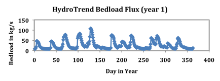
Fig. 4. Timeseries of river bedload flux to the coast as predicted by HydroTrend over a single year. This would be the first 365 values in the output file HYDROASCII.QB. The file itself will have all daily values for the entire run.

Output of the coupled model simulations after ~30 years of simulation is given as a DT_1000elevation file. These are sequences of grids (200 cells crossshore and 500 cells alongshore) of the topography and bathymetry that has been newly formed due to delta deposition. Again, any visualization software among others the VISIT sotware, that can deal with ASCII format can be used to plot these gridfiles (Matlab was used here specifically).

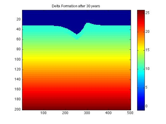
Fig. 5. Planview of the grid topography shows the subarial part of the delta built out into the marine basin. The delta growth after 29000 timesteps has been asymmetric, since the waves come in under an angle.

 

5          More Information in Model Repository

Components are described in the CSDMS model repository. Please find additional information at the following website:

http://csdms.colorado.edu/wiki/Models

Specifically there are pages for HydroTrend and CEM:

http://csdms.colorado.edu/wiki/Model:HydroTrend

http://csdms.colorado.edu/wiki/Model:CEM

 

6          References

Kettner, A.J., and Syvitski, J.P.M., 2008. HydroTrend version 3.0: a Climate-Driven Hydrological Transport Model that Simulates Discharge and Sediment Load leaving a River System. Computers & Geosciences, Special Issue.

Syvitski, J.P.M., Morehead, M.D. and Nicholson, M., 1998. HYDROTREND: A Climate-driven Hydrologic-Transport Model for Predicting Discharge and Sediment Loads to Lakes or Oceans. Computers & Geosciences, 24(1), 51-68.

Ashton, A, A.B. Murray, and O. Arnoult. 2001. "Formation of coastline features by large-scale instabilities induced by high-angle waves." Nature 414: 296-300.

Ashton, A. D. and A. B. Murray. 2006a. "High-angle wave instability and emergent shoreline shapes: 1. Modeling of sand waves, flying spits, and capes. Journal of Geophysical Research 111. F04011, doi:10.1029/2005JF000422.