Model:Plume
Plume
Introduction
PLUME [1] [2][3]
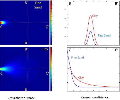
Plume simulates hypopycnal plumes generated by a river draining its suspended sediment load into a receiving basin. Satellite images of any river-delta emphasize the importance of river plumes. A plume’s behavior is dependent on the density contrast between the river water and the standing water (Albertson, 1950; Bates, 1953). Ocean water has a high density, and the plumes often flow buoyantly on the surface (hypopycnal). Another complementary model that deals with more rare hyperpycnal flows is [[Model:Sakura|Sakura]. The river’s sediment concentration adds density to the freshwater, but usually the effluent remains below the density of seawater. The shape that a hypopycnal plume will have, depends on a variety of factors:
- Angle between the river course and the coastline
- Strength and direction of the coastal current
- Wind direction influencing local upwelling or downwelling
- Mixing tidal or storm energy near the river mouth
- Latitude and thus the strength of the Coriolis effect.
The plume equations follow those of Albertson (1950) developed for a jet flowing into a steady receiving basin. Plumes of similar shape but differing concentrations result for each grain size in the model. Fine sand will generally settle rapidly, whereas clay can travel much larger distances. Naturally, this affects the geometry of the deposited sediments on the basin floor.
River dimensions, i.e. the channel width, depth and velocity at the river mouth are input conditions. In addition, river sediment concentration and settling velocities for specific grain size classes are input parameters as well. Plume is a steady-state model, meaning that it simulates constant input conditions, representative of a 'unit' event.
River dimensions for plume range over orders of magnitude, small streams of only a few meters wide have been run, as well as large continental scale rivers (for example the Ganges-Brahmaputra). Consequently, the spatial resolution of the grid is highly variable depending on the modeling objective. If plume is used in stand-alone mode, it runs events of a single day. If you are interested in exploring deposits of changing plumes over time you will need to use the PLUME model within the framework of the stratigraphic model Sedflux.
References to plume theory
Albertson, M.L., Dai, Y.B., Jensen, R.A., Hunter, R., 1950, Diffusion of submerged jets. American Society Civil Engineers Trans, v. 115, p. 639-697.
Bates, C.C., 1953, Rational theory of delta formation. AAPG Bulletin, v. 37, p. 2119-2162.
Plume model papers
- ↑ Hutton and Syvitski, 2008. Sedflux-2.0: An advanced process-response model that generates three-dimensional stratigraphy. Computers and Geosciences, v. 34. doi:10.1016/j.cageo.2008.02.013
- ↑ Syvitski et al., 1998. PLUME1.1: Deposition of sediment from a fluvial plume (doi:10.1016/S0098-3004(97)00084-8
- ↑ Peckham, S.D., 2008. A new method for estimating suspended sediment concentrations and deposition rates from satellite imagery based on the physics of plumes. Computer & Geosciences, 34, 1198-1222. doi:10.1016/j.cageo.2008.02.009
Plume Questionnaire
Contact Information
| Model: | Plume |
| Contact person: | Eric Hutton |
| Institute: | University of Colorado |
| City: | Boulder, CO |
| Country: | USA |
| Email: | -- |
Model description
| Model type: | Single model |
| Description: | Run a hypopycnal sediment plume |
Technical information
| Supported platforms: | UNIX, Linux, Mac OSX, Windows |
| Programming language: | C |
| Model was developed started from: | 1997 and development still takes place |
| To what degree will the model become available: | As code |
| Current license type: | Apache public license |
| Memory requirements: | Minimal |
| Typical run time: | seconds |
Input / Output description
| Input parameters: | River velocity, width, depth; Sediment concentrations |
| Input format: | ASCII |
| Output parameters: | Grid of Sediment rate in m/day for specified grain size classes |
| Output format: | ASCII |
| Post-processing software (if needed): | no |
| Visualization software (if needed): | no |
Process description
| Processes represented by model: | Steady-state river generated hypopycnal sediment plume |
| Key physical parameters & equations: | 2D advection-diffusion equation |
| Length scale & resolution constraints: | kilometers to tens of kilometers; resolution typically 10 to 100s of meters |
| Time scale & resolution constraints: | Daily; Steady-state |
| Numerical limitations and issues : |
Testing
| Available calibration data sets: | Eel River (California), Knight and Bute Inlet (British Columbia) |
| Available test data sets: | -- |
| Ideal data for testing: | -- |
User groups
| Currently or plans for collaborating with: | None |
Documentation
| Key papers of the model: | Syvitski et al., 1998 (doi:10.1016/S0098-3004(97)00084-8) |
| Is there a manual available: | no |
| Model website if any: | -- |
Additional comments
| Comments: | -- |
Issues
Help
Help on Model Output
PLUME generates a comma separated (*.csv) file which shows sedimentation rates per specified grain size class in m/day for the entire model grid.
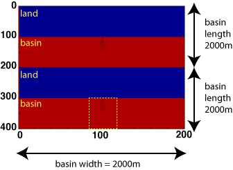
Half of the model grid is land, the other half is the receiving marine or lake basin as shown in the accompanying figure. The sedimentation rate for the first specified grainsize is listed for every gridcell. The small plume in the example is visible in the middle of the grid.
Then the grid repeats itself for the next grainsize, of which the plume has a different shape and sedimentation rate. So a grid of 2000m basin width and length, with gridcells of 10 by 10 m will have 400 rows by 200 columns, if the simulation was only run for two grain size classes.
This would repeat on to match the total number of simulated grain size classes.
Help on Simple Matlab Visualization of Output
If you want to use PLUME output with Matlab you will have to cut off the header lines of the file in a text editor. These are just a couple of commands to get started with analyzing the output.
In Matlab use the following commands:
To import your generated output file: <geshi lang=matlab> > c=dlmread('*.csv'); </geshi>
To create a planview map the plumes: <geshi lang=matlab> > imagesc(c); </geshi> Usually the first grain size is the coarser fraction traveling in suspension, but it is dependent on your input file. If you just want to create a planview map of a single grainsize plume:
<geshi lang=matlab> > cg1=c(101:200,:); > cg2=c(301:400,:); > imagesc(cg1) > figure > imagesc(cg2) </geshi>
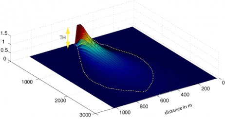
If you want the plume area of all cells with more than a certain threshold of sediment deposited, in this example all area with more than 0.005m deposits, you can get the no-of-gridcells that contain layers thicker than a certain threshold:
<geshi lang=matlab> > n=sum(sum(cg1>0.0005); > plume_area=n*10*10; </geshi>
Similarly, if you want the plume volume of all cells with more than a certain threshold of sediment deposited, in this example all area with more than 0.005m deposits, you can get the no-of-gridcells that contain layers thicker than a certain threshold:
<geshi lang=matlab> > v=sum(cg1>0.0005); > plume_volume=v*10*10; </geshi>
It may be usefull to compare X-sections for the different grain size classes: <geshi lang=matlab> > plot(cg1(25, :), 'r'); > hold > plot(cg2(25,:)); </geshi>
Input Files
Output Files
Download
Source-Code Snapshots
Source-code snapshots are available via ftp at:
The latest version:
Simple Input Files for Testing
A very simple scenario for the plume model has been posted here. It models a bankfull flood event for a small meandering river, draining into a lake. These files may be useful for testing whether the model is running.
- plume parameter file (January 2009, kvf format)
- plume flood file (January 2009, kvf format)
Simple Output File for Testing
The associated output file, with grids of sedimentation rates per day, for both grain sizes can be found here:
- plume output file (January 2009, csv format)
Source
plume is part of the sedflux model. Although it is also available as a seperate distribution, its source code is contained within the sedflux repository.
To browse the repository, point your browser to: http://csdms.colorado.edu/viewvc/sedflux/?root=sedflux
Command-Line Access
If you plan to make changes, use this command to check out the code as yourself using HTTPS:
<geshi lang=bash>
- Project members authenticate over HTTPS to allow committing changes.
svn checkout https://csdms.colorado.edu/svn/sedflux/ </geshi>
When prompted, enter your CSDMS Subversion password.
Non-members may only check out a read-only working copy of the project source.
To obtain a CSDMS Subversion account or to become a member of this project, please email csdms@colorado.edu.
GUI and IDE Access
This project's Subversion repository may be accessed using many different client programs and plug-ins. See your client's documentation for more information.
Subversion Help
For help on how to use Subversion, an excellent manual is available online at http://svnbook.red-bean.com/


