Labs WMT Permafrost KudryavtsevModel1D

Introduction to Permafrost Processes - Lesson 2 Kudryavtsev Model

Contributor(s)

Irina Overeem at CSDMS, University of Colorado.
Mark Piper at CSDMS, University of Colorado.
Kang Wang at East China Normal University.
Scott Stewart at CSDMS, University of Colorado.
Elchin Jafarov at Los Alamos National Labs.

Introduction

The Kudryavtsev et al. (1974), or Ku model, presents an approximate solution of the Stefan problem. The model provides a steady-state solution under the assumption of sinusoidal air temperature forcing. It considers snow, vegetation, and soil layers as thermal damping to variation of air temperature. The layer of soil is considered to be a homogeneous column with different thermal properties in the frozen and thawed states. The main outputs are annual maximum frozen/thaw depth and mean annual temperature at the top of permafrost (or at the base of the active layer). It can be applied over a wide variety of climatic conditions.

Classroom organization

This lab is the second in a series of introduction to permafrost process modeling, designed for inexperienced users. In this second lesson, we explore the Kudryavstev model and learn to use this model in the CSDMS Python Modeling Tool (Pymt). We implemented the Kudryavstev model (as formulated in Anisimov et al.1997). It is dubbed the Ku-model.

This series of labs is designed for inexperienced modelers to gain some experience with running a numerical model, changing model inputs, and analyzing model output. Specifically, this lab looks at what controls soil temperature and active layer thickness and compares model output with observed longterm data collected at permafrost active layer thickness monitoring sites in Fairbanks and Barrow, Alaska.

Basic theory on the Kudryavstev model is presented in these slides File:KudryavtsevModel Lecture2.pptx

This lab will likely take ~ 1,5 hours to complete in the classroom. This time assumes you now have gained some familiarity with the Pymt and have learned how to set parameters, save runs, download data and look at output. If this is not the case, either start with Lab 1 in this series, or learn how to use Pymt here. The Pymt allows you to set up simulations and run notebooks.

If you are a faculty at an academic institution, it is possible to work with us to get temporary teaching accounts. Work directly with us by emailing: csdms@colorado.edu

Learning objectives

Skills

familiarize with a basic configuration of the Kudryavstev Model for 1D (a single location).
hands-on experience with visualizing NetCDF time series with Panoply.
data to model comparisons and how to think about uncertainty in data and model output.

Topical learning objectives:

what are controls on permafrost soil temperature
what is a steady-state model
what are important parameters for calculating active layer thickness
active layer thickness evolution with climate warming in two locations in Alaska

Lab Notes

You can launch binder to directly run the Jupyter Notebook for this lab through a web browser.

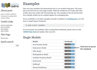
>> Open a new browser window and open the Pymt read the docs page here

>> You will see that there are several example models. In this lab we will select the Kudryatsev model.
>> Click on the 'Launch Binder' box and it will allow you to see this lab as a Jupyter Notebook.
>> You can execute the Jupyter notebook code cells using shift -enter.

Part 1

>>> We will run the Kudryatsev model for conditions in Barrow, Alaska in a very cold year, 1964. The mean annaul temperature for 1964 was -15.21C, the amplitude over that year was 18.51C. It was close to normal snow year, meaning the average snow thickness over this winter was 0.22m.

>>> Adapt the settings in the Ku model for Barrow 1964. Make sure you request an output file. Save the simulation settings and submit your simulation. Download the model results and open them in Panoply.

 Q1.1 What was the active layer thickness the model predicted? 
 Sketch a soil profile for winter conditions versus August conditions, indicate where the frozen-unfrozen boundary is in each two cases.

 Q1.2 How do you think snow affects the active layer thickness predictions?

Part 2

>> Run the Kudryatsev model with a range of snow conditions (0 m as the one extreme, and in extremely snowy years, the mean snow thickness over the winter is 0.4m in Barrow). Set these two simulations, run them and dowload the files.

Q2.1 What happens if there is no snow at all (0.0m)?

Q2.2 What is the active layer thickness prediction for a very snowy year?

Part 3

>> Run the Kudryatsev model with a range of soil water contents. What happens if there is 20% more, and 20% less soil water content?

Q3.1 Is this selected range of 20% realistic for soils in permafrost regions?

Q3.2 From the theory presented in the associated lecture notes, how do you think soil water content in summer affects the soil temperature?

Part 4

>> Posted here are time-series for climate conditions for both Barrow and Fairbanks, Alaska. Time-series are annual values and run from 1961-2015, the data include mean annual temperature (MAAT), temperature amplitude (TAMP) and winter-average snow depth (SD).

>> Download the files here, it is a zip archive and contains all six files: File:ClimateData Alaska.zip
These are text files, so you can plot them in your own favorite software or programming language.

>> Choose which case you want to run, and you will now run a 55 year simulation.

Q4.1 Is there a significant trend in the mean annual air temperature over the last 55 years?

Q4.2 Do you see a warming or cooling trend reflected in the active layer depth over time? If so, why? Or why not?

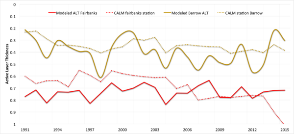
The panel above shows modeled time series for active layer thickness for both Fairbanks and Barrow, and compares these time series with observed data. The Circumarctic Active Layer Network (CALM) makes this data available.

Q4.3 Describe what you see in the data to model comparisons.

Q4.4 Why would there be a discrepancy between the model and the observations? Identify 3 possible reasons.

Q4.5 Can you design a Ku model experiment to see whether your hypotheses may be valid? Describe (or run the simulations and show it).

References

Anisimov, O. A., Shiklomanov, N. I., & Nelson, F. E. (1997). Global warming and active-layer thickness: results from transient general circulation models. Global and Planetary Change, 15(3-4), 61-77. DOI:10.1016/S0921-8181(97)00009-X
Sazonova, T.S., Romanovsky, V.E., 2003. A model for regional-scale estimation of temporal and spatial variability of active layer thickness and mean nnaual ground emperatures. Permafrost and periglacial processes 14, 125-139. DOI: 10.1002/ppp.449
Zhang, T., 2005. Influence of the seasonal snow cover on the ground thermal regime: an overview. Review of Geophysics, 43, RG4002.

More on Model code and Running this model

Documentation for this model can be found Ku Model metadata in CSDMS repository.
If you'd like to run this code independently or contribute to it, find it in our repository: Permafrost Modeling Toolbox Codes