Labs WMT Permafrost FrostNumber: Difference between revisions
mNo edit summary |
(first rough draft of pymt notebook for teaching) |
||
| Line 12: | Line 12: | ||
<br>This lab will likely take ~ 1,5 hours to complete in the classroom. This time assumes you are unfamiliar with the Pymt and need to learn setting parameters, and looking at output (otherwise it will be much faster). <br> | <br>This lab will likely take ~ 1,5 hours to complete in the classroom. This time assumes you are unfamiliar with the Pymt and need to learn setting parameters, and looking at output (otherwise it will be much faster). <br> | ||
If you have never used the Python Modeling Tool (Pymt), learn how to use it [https://pymt.readthedocs.io/en/latest/|here]. The | If you have never used the Python Modeling Tool (Pymt), learn how to use it [https://pymt.readthedocs.io/en/latest/|here]. The Pymt allows you to set up simulations, and run them and then analyze data using Python. | ||
<br> If you are a faculty at an academic institution, it is possible to work with us to get temporary teaching accounts. Work directly with us by emailing: csdms@colorado.edu | |||
'''Learning objectives'''<br> | '''Learning objectives'''<br> | ||
Skills | Skills | ||
* familiarize with a basic configuration of the Air Frost Number Model | * familiarize with a basic configuration of the Air Frost Number Model | ||
* hands-on experience with visualizing | * make small changes to key input parameters | ||
* see how to write a loop for calculations over a time series | |||
* hands-on experience with visualizing output in Python | |||
Topical learning objectives: | Topical learning objectives: | ||
| Line 27: | Line 28: | ||
* freezing and thawing day indices and how to approximate these | * freezing and thawing day indices and how to approximate these | ||
* where in Russia permafrost occurs | * where in Russia permafrost occurs | ||
* critical evaluation of what the Air Frost number approximates | |||
<br><br> | <br><br> | ||
| Line 32: | Line 34: | ||
<br> | <br> | ||
>> Open a new browser window and open the | >> Open a new browser window and open the Pymt read the docs page [https://pymt.readthedocs.io/en/latest/examples.html here] | ||
[[File: | [[File:ExampleListPymt.png|400px]] | ||
>> You will see that there are several example models. In this lab we will select the Frost number component. | |||
>> Click on the 'Launch Binder' box and it will allow you to see this lab as a Jupyter Notebook. | |||
<br><br> | <br><br> | ||
'''References and More information''' | '''References and More information''' | ||
Revision as of 16:05, 9 January 2020
Introduction to Permafrost Processes - Lesson 1 Frost Number Model
This lab has been designed and developed by Irina Overeem and Mark Piper, CSDMS, University of Colorado, CO with assistance of Kang Wang, Scott Stewart at CSDMS, University of Colorado, CO, and Elchin Jafarov, at Los Alamos National Labs, NM. These labs are developed with support from NSF Grant 1503559, ‘Towards a Tiered Permafrost Modeling Cyberinfrastructure’ and are part of the Permafrost Modeling Toolbox, https://github.com/permamodel.
Last modified by Irina Overeem: January 7th, 2020.
Classroom organization
This lab is the first in a series of introduction to permafrost process modeling, designed for inexperienced users. In this first lesson, we explore the Air Frost Number model and learn to use such models in the CSDMS Python Model tool (Pymt). We implemented a basic configuration of the Air Frost Number (as formulated by Nelson and Outcalt in 1987). This series of labs is designed for inexperienced modelers to gain some experience with running a numerical model, changing model inputs, and analyzing model output. Specifically, this first lab looks at what controls permafrost occurrence and compares the occurrence of permafrost in Russia.
Basic theory on the Air Frost Number is presented in File:FrostNumberModel Lecture1.pptx.
This lab will likely take ~ 1,5 hours to complete in the classroom. This time assumes you are unfamiliar with the Pymt and need to learn setting parameters, and looking at output (otherwise it will be much faster).
If you have never used the Python Modeling Tool (Pymt), learn how to use it [1]. The Pymt allows you to set up simulations, and run them and then analyze data using Python.
If you are a faculty at an academic institution, it is possible to work with us to get temporary teaching accounts. Work directly with us by emailing: csdms@colorado.edu
Learning objectives
Skills
- familiarize with a basic configuration of the Air Frost Number Model
- make small changes to key input parameters
- see how to write a loop for calculations over a time series
- hands-on experience with visualizing output in Python
Topical learning objectives:
- what is the primary control on the occurrence of permafrost
- freezing and thawing day indices and how to approximate these
- where in Russia permafrost occurs
- critical evaluation of what the Air Frost number approximates
Lab Notes
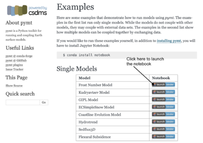
>> Open a new browser window and open the Pymt read the docs page here
>> You will see that there are several example models. In this lab we will select the Frost number component.
>> Click on the 'Launch Binder' box and it will allow you to see this lab as a Jupyter Notebook.
References and More information
- Nelson, F.E., Outcalt, S.I., 1987. A computational method for prediction and prediction and regionalization of permafrost. Arct. Alp. Res. 19, 279–288.
- Janke, J., Williams, M., Evans, A., 2012. A comparison of permafrost prediction models along a section of Trail Ridge Road, RMNP, CO. Geomorphology 138, 111-120.
More on Model code and Running this model
Documentation for this model can be found Frost_Model metadata in CSDMS repository.
If you'd like to run this code or contribute to it, find it in our repository: Permafrost Modeling Toolbox Codes

