Lab-0002

Permafrost Modeling - the Active Layer

Model
Kudryavtsev Model

Duration
1.5 hrs

Updated
2020/03/20

Download
download

Run online using:

1. Jupyter

     

This lab is part of the series Permafrost. Others in this series are:

• Permafrost Modeling - where does permafrost occur? (1 of 4)
• Permafrost Modeling - the Active Layer (2 of 4)
• Permafrost Modeling - making maps from gridded climate data (3 of 4)
• Permafrost Modeling - looking at future permafrost with climate models (4 of 4)

Contributor(s)

    Irina Overeem at CSDMS, University of Colorado.

    Mark Piper at CSDMS, University of Colorado.

    Kang Wang at East China Normal University.

    Elchin Jafarov at Los Alamos National Labs, NM.

Introduction

The Kudryavtsev et al. (1974), or Ku model, presents an approximate solution of the Stefan problem. The model provides a steady-state solution under the assumption of sinusoidal air temperature forcing. It considers snow, vegetation, and soil layers as thermal damping to variation of air temperature. The layer of soil is considered to be a homogeneous column with different thermal properties in the frozen and thawed states. The main outputs are annual maximum frozen/thaw depth and mean annual temperature at the top of permafrost (or at the base of the active layer). It can be applied over a wide variety of climatic conditions.

Classroom organization
This lab is the second in a series of introduction to permafrost process modeling, designed for inexperienced users. In this second lesson, we explore the Kudryavstev model and learn to use this model in the CSDMS Python Modeling Tool (Pymt). We implemented the Kudryavstev model (as formulated in Anisimov et al.1997). It is dubbed the Ku-model.

This series of labs is designed for inexperienced modelers to gain some experience with running a numerical model, changing model inputs, and analyzing model output. Specifically, this lab looks at what controls soil temperature and active layer thickness and compares model output with observed longterm data collected at permafrost active layer thickness monitoring sites in Fairbanks and Barrow, Alaska.

Basic theory on the Kudryavstev model is presented in these slides File:KudryavtsevModel Lecture2.pptx

This lab will likely take ~ 1,5 hours to complete in the classroom. This time assumes you now have gained some familiarity with the Pymt and have learned how to set parameters, save runs, download data and look at output. If this is not the case, either start with Lab 1 in this series, or learn how to use Pymt (https://pymt.readthedocs.io/en/latest/install.html). The Pymt allows you to set up simulations and run notebooks.

You can create an account at CSDMS JupyterHub and test the Jupyter Notebook for this lab. Please follow the instruction at: https://github.com/csdms/pymt/blob/master/notebooks/README.md. If you are a faculty at an academic institution, it is possible to work with us to get temporary teaching accounts. Work directly with us by emailing: csdms@colorado.edu

Download associated file: KudryavtsevModel Lecture2.pptx
Basic theory on the Kudryavstev model is presented in these slides

Learning objectives
Skills

• familiarize with a basic configuration of the Kudryavstev Model for 1D (a single location).
• hands-on experience with visualizing NetCDF time series with Panoply.
• data to model comparisons and how to think about uncertainty in data and model output.

Key concepts

• what are controls on permafrost soil temperature
• what is a steady-state model
• what are important parameters for calculating active layer thickness
• active layer thickness evolution with climate warming in two locations in Alaska

Lab notes

Figure 1. Screenshot of the pymt notebook

You can launch binder to directly run the Jupyter Notebook for this lab through a web browser.

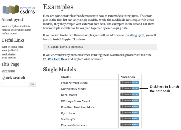
>> Open a new browser window and open the Pymt read the docs page (https://pymt.readthedocs.io/en/latest/examples.html)

>> You will see that there are several example models. In this lab we will select the Kudryatsev model.

>> Click on the 'Launch Binder' box and it will allow you to see this lab as a Jupyter Notebook.

>> You can execute the Jupyter notebook code cells using shift -enter.

Requirements
--

Acknowledgements
These labs are developed with support from NSF Grant 1503559, ‘Towards a Tiered Permafrost Modeling Cyberinfrastructure’ and are part of the Permafrost Modeling Toolbox, https://github.com/permamodel.

References

• Anisimov, O. A., Shiklomanov, N. I., & Nelson, F. E. (1997). Global warming and active-layer thickness: results from transient general circulation models. Global and Planetary Change, 15(3-4), 61-77. DOI:10.1016/S0921-8181(97)00009-X
• Sazonova, T.S., Romanovsky, V.E., 2003. A model for regional-scale estimation of temporal and spatial variability of active layer thickness and mean nnaual ground emperatures. Permafrost and periglacial processes 14, 125-139. DOI: 10.1002/ppp.449
• Zhang, T., 2005. Influence of the seasonal snow cover on the ground thermal regime: an overview. Review of Geophysics, 43, RG4002.